估計 3D 顯微影像中的異向性#

在本教學中,我們計算 3D 影像的結構張量。有關 3D 影像處理的一般介紹,請參閱 探索 3D 影像 (細胞)。我們在此使用的資料是從共軛焦螢光顯微鏡獲得的腎臟組織影像中採樣的 (更多詳細資訊請參閱 [1]kidney-tissue-fluorescence.tif 下)。

import matplotlib.pyplot as plt
import numpy as np
import plotly.express as px
import plotly.io

from skimage import data, feature

載入影像#

此生物醫學影像可透過 scikit-image 的資料登錄取得。

我們的 3D 多通道影像的形狀和大小究竟是什麼?

print(f'number of dimensions: {data.ndim}')
print(f'shape: {data.shape}')
print(f'dtype: {data.dtype}')
number of dimensions: 4
shape: (16, 512, 512, 3)
dtype: uint16

在本教學中,我們僅考慮第二個色彩通道,這為我們留下了一個 3D 單通道影像。值的範圍是多少?

n_plane, n_row, n_col, n_chan = data.shape
v_min, v_max = data[:, :, :, 1].min(), data[:, :, :, 1].max()
print(f'range: ({v_min}, {v_max})')
range: (68, 4095)

讓我們視覺化我們的 3D 影像的中間切片。

fig1 = px.imshow(
    data[n_plane // 2, :, :, 1],
    zmin=v_min,
    zmax=v_max,
    labels={'x': 'col', 'y': 'row', 'color': 'intensity'},
)

plotly.io.show(fig1)

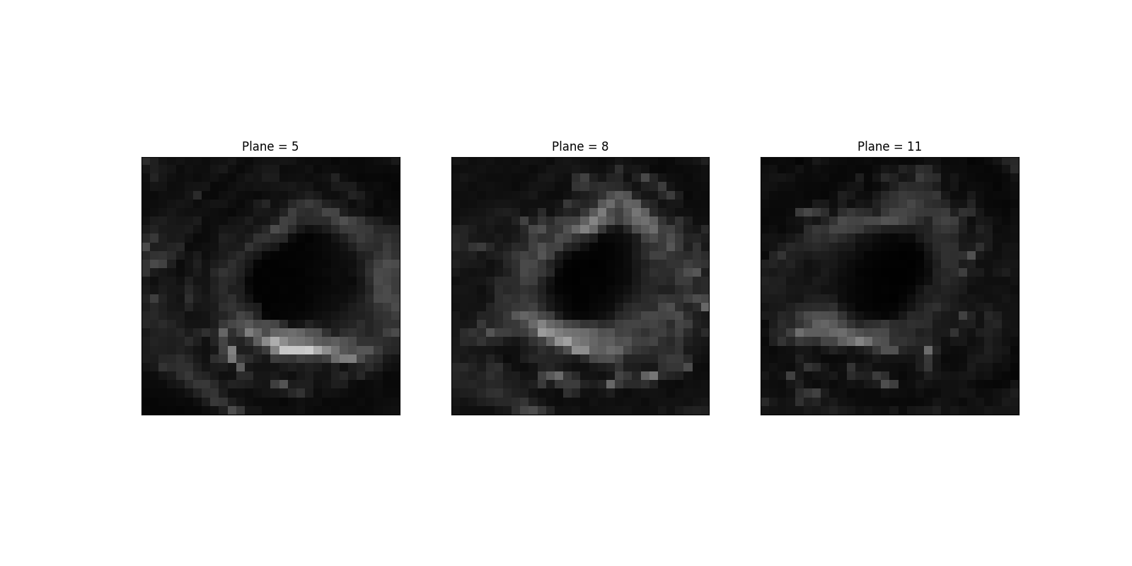
讓我們選擇一個顯示相對 X-Y 等向性的特定區域。相反地,沿著 Z 的梯度非常不同 (而且,就此而言,很弱)。

sample = data[5:13, 380:410, 370:400, 1]
step = 3
cols = sample.shape[0] // step + 1
_, axes = plt.subplots(nrows=1, ncols=cols, figsize=(16, 8))

for it, (ax, image) in enumerate(zip(axes.flatten(), sample[::step])):
    ax.imshow(image, cmap='gray', vmin=v_min, vmax=v_max)
    ax.set_title(f'Plane = {5 + it * step}')
    ax.set_xticks([])
    ax.set_yticks([])
Plane = 5, Plane = 8, Plane = 11

若要以 3D 檢視樣本資料,請執行下列程式碼

import plotly.graph_objects as go

(n_Z, n_Y, n_X) = sample.shape
Z, Y, X = np.mgrid[:n_Z, :n_Y, :n_X]

fig = go.Figure(
    data=go.Volume(
        x=X.flatten(),
        y=Y.flatten(),
        z=Z.flatten(),
        value=sample.flatten(),
        opacity=0.5,
        slices_z=dict(show=True, locations=[4])
    )
)
fig.show()

計算結構張量#

讓我們視覺化樣本資料的底部切片,並確定強烈變化的典型大小。我們應將此大小用作視窗函數的「寬度」。

fig2 = px.imshow(
    sample[0, :, :],
    zmin=v_min,
    zmax=v_max,
    labels={'x': 'col', 'y': 'row', 'color': 'intensity'},
    title='Interactive view of bottom slice of sample data.',
)

plotly.io.show(fig2)

關於最亮的區域 (即,在列 ~ 22 和欄 ~ 17 處),我們可以看到跨欄 (分別為跨列) 的 2 或 3 (分別為 1 或 2) 個像素的變化 (因此,有強烈的梯度)。因此,我們可能選擇,例如,sigma = 1.5 作為視窗函數。或者,我們可以按每個軸傳遞 sigma,例如,sigma = (1, 2, 3)。請注意,沿著第一個 (Z,平面) 軸的大小 1 聽起來很合理,因為後者的大小為 8 (13 - 5)。在 X-Z 或 Y-Z 平面中檢視切片確認這是合理的。

然後我們可以計算結構張量的特徵值。

(3, 8, 30, 30)

最大特徵值在哪裡?

coords = np.unravel_index(eigen.argmax(), eigen.shape)
assert coords[0] == 0  # by definition
coords
(np.int64(0), np.int64(1), np.int64(22), np.int64(16))

注意

讀者可以檢查此結果 (座標 (plane, row, column) = coords[1:]) 對於不同的 sigma 有多穩健。

讓我們檢視在發現最大特徵值 (即,Z = coords[1]) 的 X-Y 平面中特徵值的空間分佈。

fig3 = px.imshow(
    eigen[:, coords[1], :, :],
    facet_col=0,
    labels={'x': 'col', 'y': 'row', 'facet_col': 'rank'},
    title=f'Eigenvalues for plane Z = {coords[1]}.',
)

plotly.io.show(fig3)

我們正在查看局部屬性。讓我們考慮上述 X-Y 平面中最大特徵值附近的一個微小鄰域。

eigen[0, coords[1], coords[2] - 2 : coords[2] + 1, coords[3] - 2 : coords[3] + 1]
array([[0.05530323, 0.05929082, 0.06043806],
       [0.05922725, 0.06268274, 0.06354238],
       [0.06190861, 0.06685075, 0.06840962]])

如果我們檢查此鄰域中第二大的特徵值,我們可以發現它們與最大的特徵值具有相同的數量級。

eigen[1, coords[1], coords[2] - 2 : coords[2] + 1, coords[3] - 2 : coords[3] + 1]
array([[0.03577746, 0.03577334, 0.03447714],
       [0.03819524, 0.04172036, 0.04323701],
       [0.03139592, 0.03587025, 0.03913327]])

相反地,第三大的特徵值小一個數量級。

eigen[2, coords[1], coords[2] - 2 : coords[2] + 1, coords[3] - 2 : coords[3] + 1]
array([[0.00337661, 0.00306529, 0.00276288],
       [0.0041869 , 0.00397519, 0.00375595],
       [0.00479742, 0.00462116, 0.00442455]])

讓我們視覺化在發現最大特徵值的 X-Y 平面中樣本資料的切片。

fig4 = px.imshow(
    sample[coords[1], :, :],
    zmin=v_min,
    zmax=v_max,
    labels={'x': 'col', 'y': 'row', 'color': 'intensity'},
    title=f'Interactive view of plane Z = {coords[1]}.',
)

plotly.io.show(fig4)

讓我們視覺化在發現最大特徵值的 X-Z (左) 和 Y-Z (右) 平面中樣本資料的切片。Z 軸是下面子圖中的垂直軸。我們可以看到沿著 Z 軸的預期相對不變性 (對應於腎臟組織中的縱向結構),尤其是在 Y-Z 平面中 (longitudinal=1)。

subplots = np.dstack((sample[:, coords[2], :], sample[:, :, coords[3]]))
fig5 = px.imshow(
    subplots, zmin=v_min, zmax=v_max, facet_col=2, labels={'facet_col': 'longitudinal'}
)

plotly.io.show(fig5)

總而言之,體素 (plane, row, column) = coords[1:] 附近的區域在 3D 中是異向的:第三大的特徵值一方面和最大和第二大的特徵值另一方面之間存在一個數量級的差異。我們可以在圖表 平面 Z = 1 的特徵值 中一目了然。

有問題的鄰域在平面中是「有點各向同性」的 (在這裡,它會相對接近 X-Y 平面):第二大和最大特徵值之間存在小於 2 的因子。此描述與我們在影像中看到的相容,即,跨越方向 (在這裡,它會相對接近列軸) 的更強梯度和垂直於它的較弱梯度。

在 3D 結構張量的橢圓表示中 [2],我們會得到薄煎餅情況。

腳本的總執行時間: (0 分鐘 5.435 秒)

由 Sphinx-Gallery 產生的圖庫