使用 Haar-like 特徵描述子進行臉部分類

Haar-like 特徵描述子已成功用於實現第一個即時臉部偵測器 [1]。受此應用啟發，我們提出一個範例，說明 Haar-like 特徵的提取、選擇和分類，以偵測臉部與非臉部。

注意事項

此範例依賴於 scikit-learn 進行特徵選擇和分類。

參考文獻

[1]

Viola, Paul, and Michael J. Jones. “Robust real-time face detection.” International journal of computer vision 57.2 (2004): 137-154. https://www.merl.com/publications/docs/TR2004-043.pdf DOI:10.1109/CVPR.2001.990517

from time import time

import numpy as np
import matplotlib.pyplot as plt

from sklearn.ensemble import RandomForestClassifier
from sklearn.model_selection import train_test_split
from sklearn.metrics import roc_auc_score

from skimage.data import lfw_subset
from skimage.transform import integral_image
from skimage.feature import haar_like_feature
from skimage.feature import haar_like_feature_coord
from skimage.feature import draw_haar_like_feature

從影像中提取 Haar-like 特徵的過程相對簡單。首先，定義感興趣區域 (ROI)。其次，計算此 ROI 內的積分影像。最後，使用積分影像提取特徵。

def extract_feature_image(img, feature_type, feature_coord=None):
    """Extract the haar feature for the current image"""
    ii = integral_image(img)
    return haar_like_feature(
        ii,
        0,
        0,
        ii.shape[0],
        ii.shape[1],
        feature_type=feature_type,
        feature_coord=feature_coord,
    )

我們使用 CBCL 資料集的子集，該資料集由 100 張臉部影像和 100 張非臉部影像組成。每張影像都已調整大小為 19 x 19 像素的 ROI。我們從每組中選擇 75 張影像來訓練分類器並確定最顯著的特徵。每種類別的剩餘 25 張影像用於評估分類器的效能。

images = lfw_subset()
# To speed up the example, extract the two types of features only
feature_types = ['type-2-x', 'type-2-y']

# Compute the result
t_start = time()
X = [extract_feature_image(img, feature_types) for img in images]
X = np.stack(X)
time_full_feature_comp = time() - t_start

# Label images (100 faces and 100 non-faces)
y = np.array([1] * 100 + [0] * 100)

X_train, X_test, y_train, y_test = train_test_split(
    X, y, train_size=150, random_state=0, stratify=y
)

# Extract all possible features
feature_coord, feature_type = haar_like_feature_coord(
    width=images.shape[2], height=images.shape[1], feature_type=feature_types
)

可以訓練隨機森林分類器，以便選擇最顯著的特徵，特別是對於臉部分類。其想法是確定樹木集合最常使用哪些特徵。透過在後續步驟中僅使用最顯著的特徵，我們可以大幅加速計算速度，同時保持準確性。

# Train a random forest classifier and assess its performance
clf = RandomForestClassifier(
    n_estimators=1000, max_depth=None, max_features=100, n_jobs=-1, random_state=0
)
t_start = time()
clf.fit(X_train, y_train)
time_full_train = time() - t_start
auc_full_features = roc_auc_score(y_test, clf.predict_proba(X_test)[:, 1])

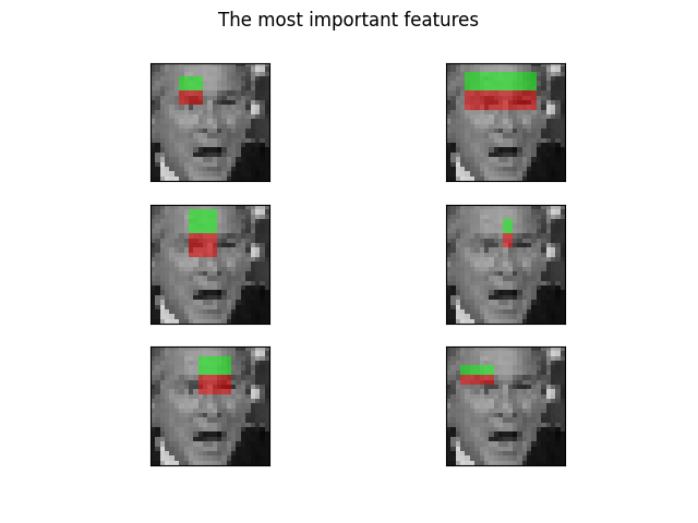
# Sort features in order of importance and plot the six most significant
idx_sorted = np.argsort(clf.feature_importances_)[::-1]

fig, axes = plt.subplots(3, 2)
for idx, ax in enumerate(axes.ravel()):
    image = images[0]
    image = draw_haar_like_feature(
        image, 0, 0, images.shape[2], images.shape[1], [feature_coord[idx_sorted[idx]]]
    )
    ax.imshow(image)
    ax.set_xticks([])
    ax.set_yticks([])

_ = fig.suptitle('The most important features')

我們可以透過檢查特徵重要性的累積總和來選擇最重要的特徵。在此範例中，我們保留代表累積值 70% 的特徵（這相當於僅使用特徵總數的 3%）。

cdf_feature_importances = np.cumsum(clf.feature_importances_[idx_sorted])
cdf_feature_importances /= cdf_feature_importances[-1]  # divide by max value
sig_feature_count = np.count_nonzero(cdf_feature_importances < 0.7)
sig_feature_percent = round(sig_feature_count / len(cdf_feature_importances) * 100, 1)
print(
    f'{sig_feature_count} features, or {sig_feature_percent}%, '
    f'account for 70% of branch points in the random forest.'
)

# Select the determined number of most informative features
feature_coord_sel = feature_coord[idx_sorted[:sig_feature_count]]
feature_type_sel = feature_type[idx_sorted[:sig_feature_count]]
# Note: it is also possible to select the features directly from the matrix X,
# but we would like to emphasize the usage of `feature_coord` and `feature_type`
# to recompute a subset of desired features.

# Compute the result
t_start = time()
X = [extract_feature_image(img, feature_type_sel, feature_coord_sel) for img in images]
X = np.stack(X)
time_subs_feature_comp = time() - t_start

y = np.array([1] * 100 + [0] * 100)
X_train, X_test, y_train, y_test = train_test_split(
    X, y, train_size=150, random_state=0, stratify=y
)

712 features, or 0.7%, account for 70% of branch points in the random forest.

提取特徵後，我們可以訓練並測試新的分類器。

t_start = time()
clf.fit(X_train, y_train)
time_subs_train = time() - t_start

auc_subs_features = roc_auc_score(y_test, clf.predict_proba(X_test)[:, 1])

summary = (
    f'Computing the full feature set took '
    f'{time_full_feature_comp:.3f}s, '
    f'plus {time_full_train:.3f}s training, '
    f'for an AUC of {auc_full_features:.2f}. '
    f'Computing the restricted feature set took '
    f'{time_subs_feature_comp:.3f}s, plus {time_subs_train:.3f}s '
    f'training, for an AUC of {auc_subs_features:.2f}.'
)

print(summary)
plt.show()

Computing the full feature set took 29.998s, plus 3.076s training, for an AUC of 1.00. Computing the restricted feature set took 0.170s, plus 2.463s training, for an AUC of 1.00.