注意
前往結尾以下載完整的範例程式碼。或透過 Binder 在您的瀏覽器中執行此範例
雷登變換#
在電腦斷層掃描中,斷層掃描重建問題是從一組投影中獲得斷層掃描切片影像[1]。投影的形成方式為:將一組平行射線穿過感興趣的 2D 物件,將物件對比沿著每條射線的積分指派給投影中的單個像素。2D 物件的單個投影是一維的。為了能夠對物件進行電腦斷層掃描重建,必須取得多個投影,每個投影對應於射線相對於物件的不同角度。在多個角度下的投影集合稱為正弦圖,它是原始影像的線性變換。
反雷登變換用於電腦斷層掃描中,以從測量的投影(正弦圖)重建 2D 影像。反雷登變換的實用、精確實作不存在,但有幾個可用的良好近似演算法。
由於反雷登變換從一組投影重建物件,因此(正向)雷登變換可用於模擬斷層掃描實驗。
此腳本執行雷登變換以模擬斷層掃描實驗,並根據模擬形成的正弦圖重建輸入影像。比較了兩種執行反雷登變換和重建原始影像的方法:濾波反投影 (FBP) 和同步代數重建技術 (SART)。
有關斷層掃描重建的更多資訊,請參閱
正向變換#
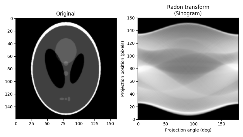
作為我們的原始影像,我們將使用 Shepp-Logan 幻影。在計算雷登變換時,我們需要決定要使用多少個投影角度。根據經驗,投影數量應與物件的像素數量大致相同(若要了解原因,請考量在重建過程中必須確定的未知像素值數量,並將其與投影提供的測量數量進行比較),而我們在此遵循該規則。以下是原始影像及其雷登變換,通常稱為其正弦圖
import numpy as np
import matplotlib.pyplot as plt

from skimage.data import shepp_logan_phantom
from skimage.transform import radon, rescale

image = shepp_logan_phantom()
image = rescale(image, scale=0.4, mode='reflect', channel_axis=None)

fig, (ax1, ax2) = plt.subplots(1, 2, figsize=(8, 4.5))

ax1.set_title("Original")
ax1.imshow(image, cmap=plt.cm.Greys_r)

theta = np.linspace(0.0, 180.0, max(image.shape), endpoint=False)
sinogram = radon(image, theta=theta)
dx, dy = 0.5 * 180.0 / max(image.shape), 0.5 / sinogram.shape[0]
ax2.set_title("Radon transform\n(Sinogram)")
ax2.set_xlabel("Projection angle (deg)")
ax2.set_ylabel("Projection position (pixels)")
ax2.imshow(
    sinogram,
    cmap=plt.cm.Greys_r,
    extent=(-dx, 180.0 + dx, -dy, sinogram.shape[0] + dy),
    aspect='auto',
)

fig.tight_layout()
plt.show()
使用濾波反投影 (FBP) 進行重建#
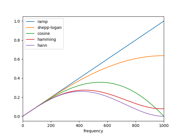
濾波反投影的數學基礎是傅立葉切片定理[2]。它使用投影的傅立葉變換和傅立葉空間中的內插來獲得影像的 2D 傅立葉變換,然後將其反轉以形成重建影像。濾波反投影是執行反雷登變換的最快方法之一。FBP 的唯一可調整參數是濾波器,它會套用至傅立葉轉換後的投影。它可用於抑制重建中的高頻雜訊。skimage 提供「ramp」、「shepp-logan」、「cosine」、「hamming」和「hann」濾波器
import matplotlib.pyplot as plt
from skimage.transform.radon_transform import _get_fourier_filter

filters = ['ramp', 'shepp-logan', 'cosine', 'hamming', 'hann']

for ix, f in enumerate(filters):
    response = _get_fourier_filter(2000, f)
    plt.plot(response, label=f)

plt.xlim([0, 1000])
plt.xlabel('frequency')
plt.legend()
plt.show()
使用「ramp」濾波器套用反雷登變換,我們得到
from skimage.transform import iradon

reconstruction_fbp = iradon(sinogram, theta=theta, filter_name='ramp')
error = reconstruction_fbp - image
print(f'FBP rms reconstruction error: {np.sqrt(np.mean(error**2)):.3g}')

imkwargs = dict(vmin=-0.2, vmax=0.2)
fig, (ax1, ax2) = plt.subplots(1, 2, figsize=(8, 4.5), sharex=True, sharey=True)
ax1.set_title("Reconstruction\nFiltered back projection")
ax1.imshow(reconstruction_fbp, cmap=plt.cm.Greys_r)
ax2.set_title("Reconstruction error\nFiltered back projection")
ax2.imshow(reconstruction_fbp - image, cmap=plt.cm.Greys_r, **imkwargs)
plt.show()
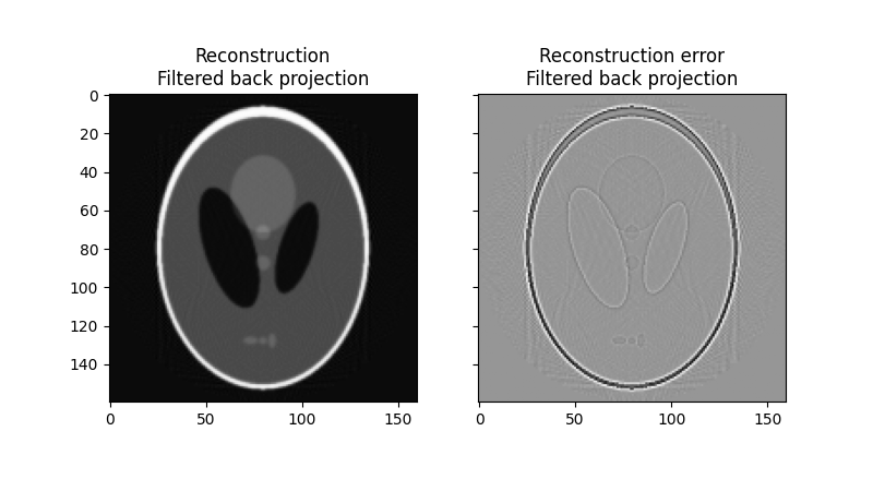
FBP rms reconstruction error: 0.0283
使用同步代數重建技術進行重建#
斷層掃描的代數重建技術基於一個簡單的想法:對於像素化影像,特定投影中單條射線的值只是射線在穿過物件的路徑上所通過的所有像素的總和。這是表達正向雷登變換的一種方式。然後,反雷登變換可以公式化為一組(大型)線性方程式。由於每條射線都穿過影像中的一小部分像素,因此這組方程式是稀疏的,因此允許稀疏線性系統的迭代解算器來解決方程式系統。有一種迭代方法特別受歡迎,即卡茲馬茲方法[3],它的特性是解法會接近方程式集的最小平方解。
將重建問題公式化為一組線性方程式和迭代解算器的組合,使代數技術相對靈活,因此可以相對容易地納入某些形式的先驗知識。
skimage 提供代數重建技術中較為流行的變體之一:同步代數重建技術 (SART) [4]。它使用卡茲馬茲方法作為迭代解算器。通常在單次迭代中獲得良好的重建,使該方法在計算上有效。執行一個或多個額外迭代通常會改善尖銳高頻特徵的重建,並減少均方誤差,但會增加高頻雜訊(使用者需要決定哪種迭代次數最適合手邊的問題。 skimage 中的實作允許將重建值的下限和上限形式的先驗資訊提供給重建。
from skimage.transform import iradon_sart

reconstruction_sart = iradon_sart(sinogram, theta=theta)
error = reconstruction_sart - image
print(
    f'SART (1 iteration) rms reconstruction error: ' f'{np.sqrt(np.mean(error**2)):.3g}'
)

fig, axes = plt.subplots(2, 2, figsize=(8, 8.5), sharex=True, sharey=True)
ax = axes.ravel()

ax[0].set_title("Reconstruction\nSART")
ax[0].imshow(reconstruction_sart, cmap=plt.cm.Greys_r)

ax[1].set_title("Reconstruction error\nSART")
ax[1].imshow(reconstruction_sart - image, cmap=plt.cm.Greys_r, **imkwargs)

# Run a second iteration of SART by supplying the reconstruction
# from the first iteration as an initial estimate
reconstruction_sart2 = iradon_sart(sinogram, theta=theta, image=reconstruction_sart)
error = reconstruction_sart2 - image
print(
    f'SART (2 iterations) rms reconstruction error: '
    f'{np.sqrt(np.mean(error**2)):.3g}'
)

ax[2].set_title("Reconstruction\nSART, 2 iterations")
ax[2].imshow(reconstruction_sart2, cmap=plt.cm.Greys_r)

ax[3].set_title("Reconstruction error\nSART, 2 iterations")
ax[3].imshow(reconstruction_sart2 - image, cmap=plt.cm.Greys_r, **imkwargs)
plt.show()
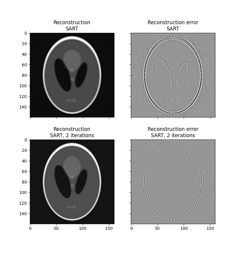
SART (1 iteration) rms reconstruction error: 0.0329
SART (2 iterations) rms reconstruction error: 0.0214
腳本總執行時間: (0 分鐘 2.276 秒)