形狀索引

形狀索引是局部曲率的單一數值度量，從黑塞矩陣的特徵值導出，由 Koenderink & van Doorn 定義 [1]。

它可用於根據結構的明顯局部形狀尋找結構。

形狀索引映射到 -1 到 1 的值，代表不同種類的形狀（詳情請參閱文件）。

在此範例中，會產生帶有斑點的隨機影像，應該偵測這些斑點。

形狀索引 1 代表「球形帽」，也就是我們要偵測的斑點形狀。

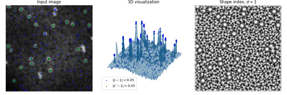
最左邊的圖顯示產生的影像，中間顯示影像的 3D 渲染，將強度值作為 3D 表面的高度，右邊的圖顯示形狀索引 (s)。

如可見，形狀索引也很容易放大雜訊的局部形狀，但不受整體現象（例如，不均勻照明）的影響。

藍色和綠色標記是偏離所需形狀不超過 0.05 的點。為了衰減訊號中的雜訊，綠色標記取自經過另一次高斯模糊處理後（產生 s'）的形狀索引 (s)。

請注意，太過緊密連接的斑點不會被偵測到，因為它們不具備所需的形狀。

[1]

Koenderink, J. J. & van Doorn, A. J., “Surface shape and curvature scales”, Image and Vision Computing, 1992, 10, 557-564. DOI:10.1016/0262-8856(92)90076-F

import numpy as np
import matplotlib.pyplot as plt
from scipy import ndimage as ndi
from skimage.feature import shape_index
from skimage.draw import disk


def create_test_image(image_size=256, spot_count=30, spot_radius=5, cloud_noise_size=4):
    """
    Generate a test image with random noise, uneven illumination and spots.
    """
    rng = np.random.default_rng()
    image = rng.normal(loc=0.25, scale=0.25, size=(image_size, image_size))

    for _ in range(spot_count):
        rr, cc = disk(
            (rng.integers(image.shape[0]), rng.integers(image.shape[1])),
            spot_radius,
            shape=image.shape,
        )
        image[rr, cc] = 1

    image *= rng.normal(loc=1.0, scale=0.1, size=image.shape)

    image *= ndi.zoom(
        rng.normal(loc=1.0, scale=0.5, size=(cloud_noise_size, cloud_noise_size)),
        image_size / cloud_noise_size,
    )

    return ndi.gaussian_filter(image, sigma=2.0)


# First create the test image and its shape index

image = create_test_image()

s = shape_index(image)

# In this example we want to detect 'spherical caps',
# so we threshold the shape index map to
# find points which are 'spherical caps' (~1)

target = 1
delta = 0.05

point_y, point_x = np.where(np.abs(s - target) < delta)
point_z = image[point_y, point_x]

# The shape index map relentlessly produces the shape, even that of noise.
# In order to reduce the impact of noise, we apply a Gaussian filter to it,
# and show the results once in

s_smooth = ndi.gaussian_filter(s, sigma=0.5)

point_y_s, point_x_s = np.where(np.abs(s_smooth - target) < delta)
point_z_s = image[point_y_s, point_x_s]


fig = plt.figure(figsize=(12, 4))
ax1 = fig.add_subplot(1, 3, 1)

ax1.imshow(image, cmap=plt.cm.gray)
ax1.axis('off')
ax1.set_title('Input image')

scatter_settings = dict(alpha=0.75, s=10, linewidths=0)

ax1.scatter(point_x, point_y, color='blue', **scatter_settings)
ax1.scatter(point_x_s, point_y_s, color='green', **scatter_settings)

ax2 = fig.add_subplot(1, 3, 2, projection='3d', sharex=ax1, sharey=ax1)

x, y = np.meshgrid(np.arange(0, image.shape[0], 1), np.arange(0, image.shape[1], 1))

ax2.plot_surface(x, y, image, linewidth=0, alpha=0.5)

ax2.scatter(
    point_x, point_y, point_z, color='blue', label='$|s - 1|<0.05$', **scatter_settings
)

ax2.scatter(
    point_x_s,
    point_y_s,
    point_z_s,
    color='green',
    label='$|s\' - 1|<0.05$',
    **scatter_settings,
)

ax2.legend(loc='lower left')

ax2.axis('off')
ax2.set_title('3D visualization')

ax3 = fig.add_subplot(1, 3, 3, sharex=ax1, sharey=ax1)

ax3.imshow(s, cmap=plt.cm.gray)
ax3.axis('off')
ax3.set_title(r'Shape index, $\sigma=1$')

fig.tight_layout()

plt.show()