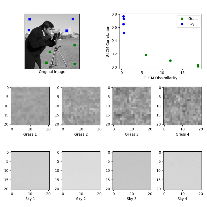
GLCM 紋理特徵

此範例說明使用灰階共生矩陣 (GLCM) [1] 的紋理分類。GLCM 是影像中給定偏移量下同時出現的灰階值的直方圖。

在此範例中，從影像中提取兩個不同紋理的樣本：草地區域和天空區域。對於每個區塊，計算水平偏移量為 5 ( distance=[5] 和 angles=[0]) 的 GLCM。接下來，計算 GLCM 矩陣的兩個特徵：差異性和相關性。繪製這些圖以說明類別在特徵空間中形成集群。在典型的分類問題中，最後一步 (不包括在此範例中) 是訓練分類器 (例如邏輯迴歸) 來標記新影像中的影像區塊。

在 0.19 版中變更： greymatrix 在 0.19 版中已重新命名為 graymatrix。

在 0.19 版中變更： greycoprops 在 0.19 版中已重新命名為 graycoprops。

參考文獻

[1]

Haralick, RM.; Shanmugam, K., "用於影像分類的紋理特徵" IEEE Transactions on systems, man, and cybernetics 6 (1973): 610-621. DOI:10.1109/TSMC.1973.4309314

import matplotlib.pyplot as plt

from skimage.feature import graycomatrix, graycoprops
from skimage import data


PATCH_SIZE = 21

# open the camera image
image = data.camera()

# select some patches from grassy areas of the image
grass_locations = [(280, 454), (342, 223), (444, 192), (455, 455)]
grass_patches = []
for loc in grass_locations:
    grass_patches.append(
        image[loc[0] : loc[0] + PATCH_SIZE, loc[1] : loc[1] + PATCH_SIZE]
    )

# select some patches from sky areas of the image
sky_locations = [(38, 34), (139, 28), (37, 437), (145, 379)]
sky_patches = []
for loc in sky_locations:
    sky_patches.append(
        image[loc[0] : loc[0] + PATCH_SIZE, loc[1] : loc[1] + PATCH_SIZE]
    )

# compute some GLCM properties each patch
xs = []
ys = []
for patch in grass_patches + sky_patches:
    glcm = graycomatrix(
        patch, distances=[5], angles=[0], levels=256, symmetric=True, normed=True
    )
    xs.append(graycoprops(glcm, 'dissimilarity')[0, 0])
    ys.append(graycoprops(glcm, 'correlation')[0, 0])

# create the figure
fig = plt.figure(figsize=(8, 8))

# display original image with locations of patches
ax = fig.add_subplot(3, 2, 1)
ax.imshow(image, cmap=plt.cm.gray, vmin=0, vmax=255)
for y, x in grass_locations:
    ax.plot(x + PATCH_SIZE / 2, y + PATCH_SIZE / 2, 'gs')
for y, x in sky_locations:
    ax.plot(x + PATCH_SIZE / 2, y + PATCH_SIZE / 2, 'bs')
ax.set_xlabel('Original Image')
ax.set_xticks([])
ax.set_yticks([])
ax.axis('image')

# for each patch, plot (dissimilarity, correlation)
ax = fig.add_subplot(3, 2, 2)
ax.plot(xs[: len(grass_patches)], ys[: len(grass_patches)], 'go', label='Grass')
ax.plot(xs[len(grass_patches) :], ys[len(grass_patches) :], 'bo', label='Sky')
ax.set_xlabel('GLCM Dissimilarity')
ax.set_ylabel('GLCM Correlation')
ax.legend()

# display the image patches
for i, patch in enumerate(grass_patches):
    ax = fig.add_subplot(3, len(grass_patches), len(grass_patches) * 1 + i + 1)
    ax.imshow(patch, cmap=plt.cm.gray, vmin=0, vmax=255)
    ax.set_xlabel(f"Grass {i + 1}")

for i, patch in enumerate(sky_patches):
    ax = fig.add_subplot(3, len(sky_patches), len(sky_patches) * 2 + i + 1)
    ax.imshow(patch, cmap=plt.cm.gray, vmin=0, vmax=255)
    ax.set_xlabel(f"Sky {i + 1}")


# display the patches and plot
fig.suptitle('Grey level co-occurrence matrix features', fontsize=14, y=1.05)
plt.tight_layout()
plt.show()