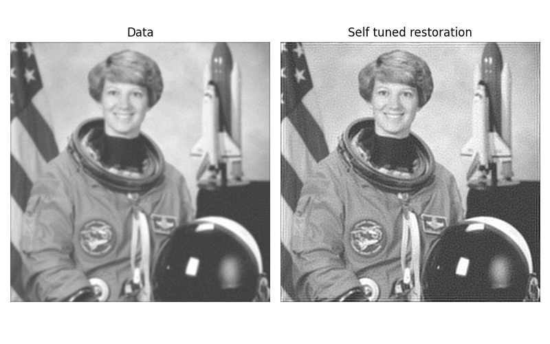
影像反褶積

在此範例中，我們使用 Wiener 和無監督 Wiener 演算法對影像的雜訊版本進行反褶積。這些演算法基於線性模型，無法像非線性方法（如 TV 復原）一樣恢復銳利的邊緣，但速度快得多。

Wiener 濾波器

基於 PSF（點擴散函數）的逆濾波器、先驗正則化（高頻率的懲罰）以及資料和先驗充分性之間的權衡。必須手動調整正則化參數。

無監督 Wiener

此演算法具有基於資料學習的自我調整正則化參數。這並不常見，並且基於以下出版物 [1]。該演算法基於迭代 Gibbs 取樣器，該取樣器交替繪製影像後驗條件定律的樣本、雜訊功率和影像頻率功率。

[1]

François Orieux, Jean-François Giovannelli, and Thomas Rodet, “Bayesian estimation of regularization and point spread function parameters for Wiener-Hunt deconvolution”, J. Opt. Soc. Am. A 27, 1593-1607 (2010) https://www.osapublishing.org/josaa/abstract.cfm?URI=josaa-27-7-1593 https://hal.archives-ouvertes.fr/hal-00674508

import numpy as np
import matplotlib.pyplot as plt

from skimage import color, data, restoration

rng = np.random.default_rng()

astro = color.rgb2gray(data.astronaut())
from scipy.signal import convolve2d as conv2

psf = np.ones((5, 5)) / 25
astro = conv2(astro, psf, 'same')
astro += 0.1 * astro.std() * rng.standard_normal(astro.shape)

deconvolved, _ = restoration.unsupervised_wiener(astro, psf)

fig, ax = plt.subplots(nrows=1, ncols=2, figsize=(8, 5), sharex=True, sharey=True)

plt.gray()

ax[0].imshow(astro, vmin=deconvolved.min(), vmax=deconvolved.max())
ax[0].axis('off')
ax[0].set_title('Data')

ax[1].imshow(deconvolved)
ax[1].axis('off')
ax[1].set_title('Self tuned restoration')

fig.tight_layout()

plt.show()