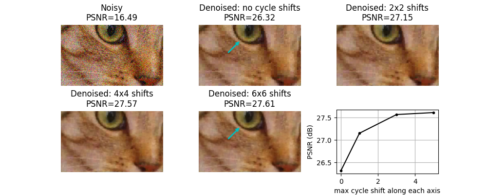
平移不變小波去噪

離散小波轉換不是平移不變的。平移不變性可以透過非抽取小波轉換（也稱為靜態小波轉換）實現，但代價是增加了冗餘度（即，小波係數多於輸入影像像素）。另一種在離散小波轉換影像去噪中逼近平移不變性的方法是使用稱為「循環旋轉」的技術。這涉及針對多個空間偏移 n，平均以下 3 步驟程序的結果：

1. 將訊號（循環）偏移量 n

2. 套用去噪

3. 套用反向偏移

對於 2D 影像去噪，我們在此展示這種循環旋轉可以顯著提高品質，而大部分增益僅僅是透過平均每個軸上僅 n=0 和 n=1 的偏移量來實現的。

Clipping input data to the valid range for imshow with RGB data ([0..1] for floats or [0..255] for integers). Got range [-0.020569158406717254..0.8458827689308539].

import matplotlib.pyplot as plt

from skimage.restoration import denoise_wavelet, cycle_spin
from skimage import data, img_as_float
from skimage.util import random_noise
from skimage.metrics import peak_signal_noise_ratio


original = img_as_float(data.chelsea()[100:250, 50:300])

sigma = 0.155
noisy = random_noise(original, var=sigma**2)

fig, ax = plt.subplots(nrows=2, ncols=3, figsize=(10, 4), sharex=False, sharey=False)
ax = ax.ravel()

psnr_noisy = peak_signal_noise_ratio(original, noisy)
ax[0].imshow(noisy)
ax[0].axis('off')
ax[0].set_title(f'Noisy\nPSNR={psnr_noisy:0.4g}')


# Repeat denosing with different amounts of cycle spinning.  e.g.
# max_shift = 0 -> no cycle spinning
# max_shift = 1 -> shifts of (0, 1) along each axis
# max_shift = 3 -> shifts of (0, 1, 2, 3) along each axis
# etc...

denoise_kwargs = dict(
    channel_axis=-1, convert2ycbcr=True, wavelet='db1', rescale_sigma=True
)

all_psnr = []
max_shifts = [0, 1, 3, 5]
for n, s in enumerate(max_shifts):
    im_bayescs = cycle_spin(
        noisy,
        func=denoise_wavelet,
        max_shifts=s,
        func_kw=denoise_kwargs,
        channel_axis=-1,
    )
    ax[n + 1].imshow(im_bayescs)
    ax[n + 1].axis('off')
    psnr = peak_signal_noise_ratio(original, im_bayescs)
    if s == 0:
        ax[n + 1].set_title(f'Denoised: no cycle shifts\nPSNR={psnr:0.4g}')
    else:
        ax[n + 1].set_title(f'Denoised: {s+1}x{s+1} shifts\nPSNR={psnr:0.4g}')
    all_psnr.append(psnr)

# plot PSNR as a function of the degree of cycle shifting
ax[5].plot(max_shifts, all_psnr, 'k.-')
ax[5].set_ylabel('PSNR (dB)')
ax[5].set_xlabel('max cycle shift along each axis')
ax[5].grid(True)
plt.subplots_adjust(wspace=0.35, hspace=0.35)

# Annotate with a cyan arrow on the 6x6 case vs. no cycle shift case to
# illustrate a region with reduced block-like artifact with cycle shifting
arrowprops = dict(
    arrowstyle="simple,tail_width=0.1,head_width=0.5", connectionstyle="arc3", color='c'
)
for i in [1, 4]:
    ax[i].annotate(
        "",
        xy=(101, 39),
        xycoords='data',
        xytext=(70, 70),
        textcoords='data',
        arrowprops=arrowprops,
    )

plt.show()