使用滾球演算法估計背景強度

滾球演算法在曝光不均勻的情況下估計灰階影像的背景強度。它常被用於生物醫學影像處理，並由 Stanley R. Sternberg 於 1983 年首次提出 [1]。

該演算法作為一個濾波器運作，而且非常直觀。我們將影像視為一個表面，每個像素的位置上都堆疊著單位大小的區塊。區塊的數量，也就是表面高度，由像素的強度決定。為了獲得所需（像素）位置的背景強度，我們想像在所需位置將一個球體浸沒在表面下方。一旦它完全被區塊覆蓋，球體的頂點就決定了該位置的背景強度。然後，我們可以將這個球體在表面下滾動，以獲得整個影像的背景值。

Scikit-image 實作了此滾球演算法的通用版本，它不僅允許您使用球體，還可以使用任意形狀作為核心，並且適用於 n 維 ndimage。這允許您直接過濾 RGB 影像或沿任何（或所有）空間維度過濾影像堆疊。

[1]

Sternberg, Stanley R. “Biomedical image processing.” Computer 1 (1983): 22-34. DOI:10.1109/MC.1983.1654163

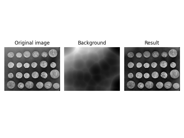
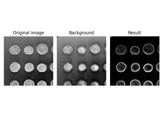
經典滾球

在 scikit-image 中，滾球演算法假設您的背景具有低強度（黑色），而特徵具有高強度（白色）。如果您的影像屬於這種情況，您可以直接使用如下的濾波器

import matplotlib.pyplot as plt
import numpy as np
import pywt

from skimage import data, restoration, util


def plot_result(image, background):
    fig, ax = plt.subplots(nrows=1, ncols=3)

    ax[0].imshow(image, cmap='gray')
    ax[0].set_title('Original image')
    ax[0].axis('off')

    ax[1].imshow(background, cmap='gray')
    ax[1].set_title('Background')
    ax[1].axis('off')

    ax[2].imshow(image - background, cmap='gray')
    ax[2].set_title('Result')
    ax[2].axis('off')

    fig.tight_layout()


image = data.coins()

background = restoration.rolling_ball(image)

plot_result(image, background)
plt.show()

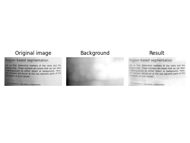
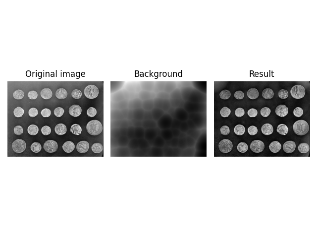
白色背景

如果您在明亮的背景上有暗色特徵，則需要在將影像傳遞到演算法之前反轉影像，然後反轉結果。這可以透過以下方式完成

image = data.page()
image_inverted = util.invert(image)

background_inverted = restoration.rolling_ball(image_inverted, radius=45)
filtered_image_inverted = image_inverted - background_inverted
filtered_image = util.invert(filtered_image_inverted)
background = util.invert(background_inverted)

fig, ax = plt.subplots(nrows=1, ncols=3)

ax[0].imshow(image, cmap='gray')
ax[0].set_title('Original image')
ax[0].axis('off')

ax[1].imshow(background, cmap='gray')
ax[1].set_title('Background')
ax[1].axis('off')

ax[2].imshow(filtered_image, cmap='gray')
ax[2].set_title('Result')
ax[2].axis('off')

fig.tight_layout()

plt.show()

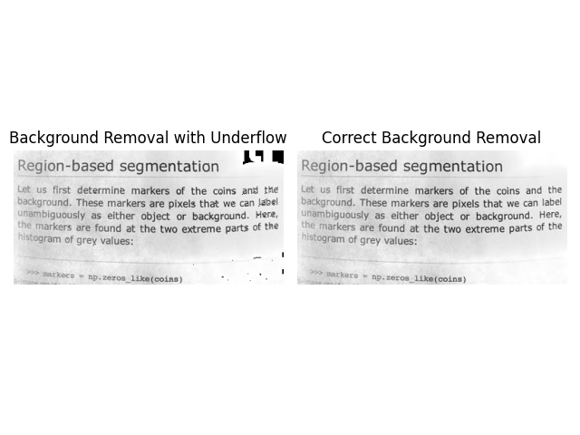
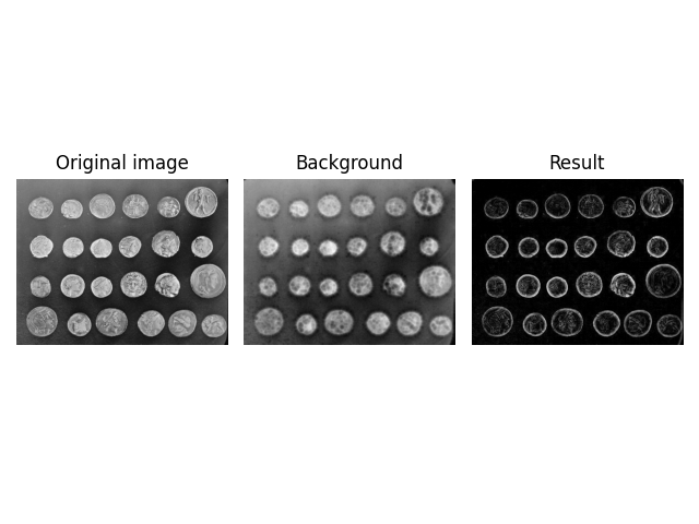
當減去明亮的背景時，請小心不要成為整數下溢的受害者。例如，此程式碼看起來正確，但可能會因下溢而導致不必要的偽影。您可以在視覺化的右上角看到這一點。

image = data.page()
image_inverted = util.invert(image)

background_inverted = restoration.rolling_ball(image_inverted, radius=45)
background = util.invert(background_inverted)
underflow_image = image - background  # integer underflow occurs here

# correct subtraction
correct_image = util.invert(image_inverted - background_inverted)

fig, ax = plt.subplots(nrows=1, ncols=2)

ax[0].imshow(underflow_image, cmap='gray')
ax[0].set_title('Background Removal with Underflow')
ax[0].axis('off')

ax[1].imshow(correct_image, cmap='gray')
ax[1].set_title('Correct Background Removal')
ax[1].axis('off')

fig.tight_layout()

plt.show()

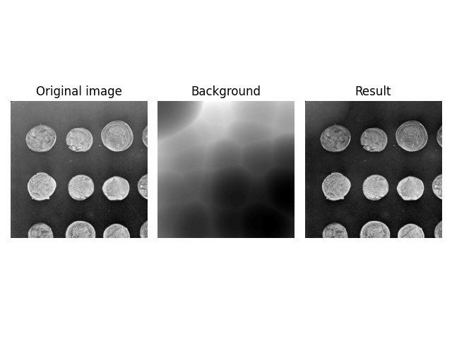
影像資料類型

rolling_ball 可以處理 np.uint8 以外的資料類型。您可以透過相同的方式將它們傳遞到函式中。

image = data.coins()[:200, :200].astype(np.uint16)

background = restoration.rolling_ball(image, radius=70.5)
plot_result(image, background)
plt.show()

但是，如果您使用已正規化為 [0, 1] 的浮點影像，則需要小心。在這種情況下，球體會比影像強度大得多，這可能會導致意外的結果。

image = util.img_as_float(data.coins()[:200, :200])

background = restoration.rolling_ball(image, radius=70.5)
plot_result(image, background)
plt.show()

由於 radius=70.5 比影像的最大強度大得多，因此有效核心大小會顯著縮小，也就是說，只有球體的一小部分（大約 radius=10）會在影像中滾動。您可以在下方的 進階形狀 部分中找到這種奇怪效果的再現。

為了獲得預期的結果，您需要降低核心的強度。這是透過使用 kernel 引數手動指定核心來完成的。

注意：半徑等於橢圓半軸的長度，它是完整軸的一半。因此，核心形狀乘以二。

normalized_radius = 70.5 / 255
image = util.img_as_float(data.coins())
kernel = restoration.ellipsoid_kernel((70.5 * 2, 70.5 * 2), normalized_radius * 2)

background = restoration.rolling_ball(image, kernel=kernel)
plot_result(image, background)
plt.show()

進階形狀

預設情況下，rolling_ball 使用球形核心（不意外）。有時，這可能會過於限制——如上面的範例所示——因為強度維度與空間維度相比具有不同的尺度，或者因為影像維度可能具有不同的含義——一個維度可能是影像堆疊中的堆疊計數器。

為了處理這種情況，rolling_ball 具有 kernel 引數，可讓您指定要使用的核心。核心的維度必須與影像的維度相同（注意：是維度，而不是形狀）。為了幫助建立核心，skimage 提供了兩個預設核心。ball_kernel 指定球形核心，並用作預設核心。ellipsoid_kernel 指定橢圓體形核心。

image = data.coins()
kernel = restoration.ellipsoid_kernel((70.5 * 2, 70.5 * 2), 70.5 * 2)

background = restoration.rolling_ball(image, kernel=kernel)
plot_result(image, background)
plt.show()

您也可以使用 ellipsoid_kernel 重現先前出乎意料的結果，並查看有效（空間）濾波器大小已縮小。

image = data.coins()

kernel = restoration.ellipsoid_kernel((10 * 2, 10 * 2), 255 * 2)

background = restoration.rolling_ball(image, kernel=kernel)
plot_result(image, background)
plt.show()

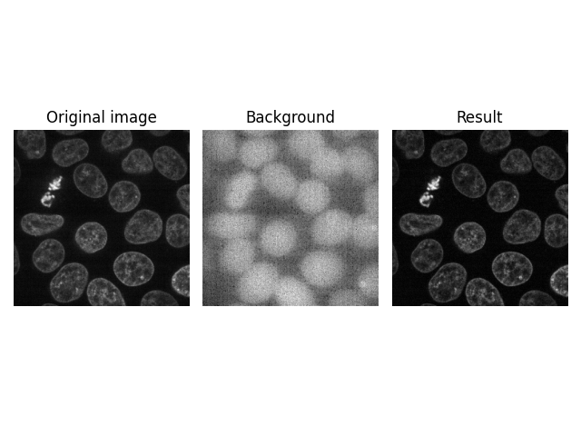
更高維度

rolling_ball 的另一個特點是您可以將其直接應用於更高維度的影像，例如，在共軛焦顯微鏡中獲得的影像 z 軸堆疊。核心維度的數量必須與影像維度匹配，因此核心形狀現在是 3 維的。

image = data.cells3d()[:, 1, ...]
background = restoration.rolling_ball(
    image, kernel=restoration.ellipsoid_kernel((1, 21, 21), 0.1)
)

plot_result(image[30, ...], background[30, ...])
plt.show()

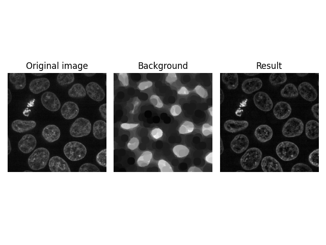
核心大小為 1 時，不會沿此軸進行過濾。換句話說，上面的濾波器會單獨應用於堆疊中的每個影像。

但是，您也可以透過指定 1 以外的值，同時沿所有 3 個維度進行過濾。

image = data.cells3d()[:, 1, ...]
background = restoration.rolling_ball(
    image, kernel=restoration.ellipsoid_kernel((5, 21, 21), 0.1)
)

plot_result(image[30, ...], background[30, ...])
plt.show()

另一種可能性是沿平面軸（z 軸堆疊）過濾單獨的像素。

image = data.cells3d()[:, 1, ...]
background = restoration.rolling_ball(
    image, kernel=restoration.ellipsoid_kernel((100, 1, 1), 0.1)
)

plot_result(image[30, ...], background[30, ...])
plt.show()

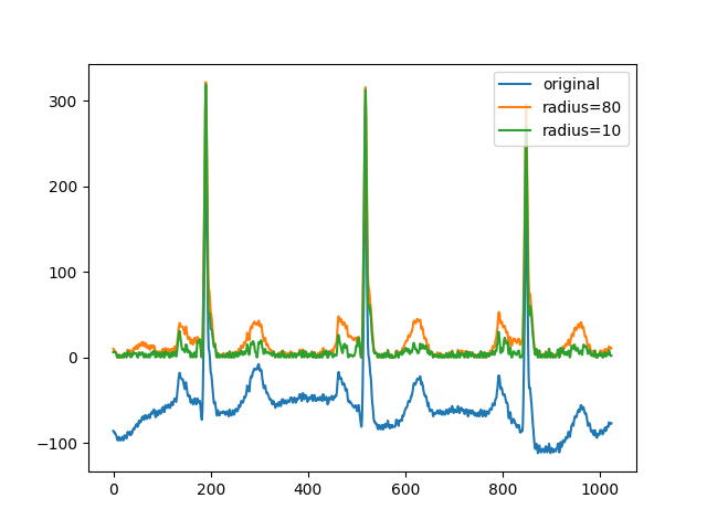
一維訊號濾波

作為 rolling_ball 的 n 維功能的另一個範例，我們展示了 1 維資料的實作。在這裡，我們感興趣的是去除心電圖波形的背景訊號，以檢測突出的波峰（高於局部基準線的值）。可以使用較小的半徑值去除較平滑的波峰。

x = pywt.data.ecg()
background = restoration.rolling_ball(x, radius=80)
background2 = restoration.rolling_ball(x, radius=10)
plt.figure()
plt.plot(x, label='original')
plt.plot(x - background, label='radius=80')
plt.plot(x - background2, label='radius=10')
plt.legend()
plt.show()