使用修復技術還原帶有斑點的角膜影像

光學同調斷層掃描 (OCT) 是一種由眼科醫生使用，用於拍攝患者眼後部的非侵入性影像技術 [1]。在執行 OCT 時，灰塵可能會黏在設備的參考鏡上，導致影像上出現黑點。問題是這些污垢點覆蓋了體內組織的區域，因此隱藏了感興趣的資料。我們這裡的目標是根據邊界附近的像素來還原（重建）隱藏區域。

本教學改編自 Jules Scholler 分享的應用程式 [2]。這些影像是由 Viacheslav Mazlin 獲取的（請參閱 skimage.data.palisades_of_vogt()）。

[1]

David Turbert，由 Ninel Z Gregori，MD 審閱 (2023) 什麼是光學同調斷層掃描？，美國眼科學院。

[2]

Jules Scholler (2019)「使用修復技術進行影像去噪」https://www.jscholler.com/2019-02-28-remove-dots/

import matplotlib.pyplot as plt
import numpy as np
import plotly.io
import plotly.express as px

import skimage as ski

我們在這裡使用的資料集是人類體內組織的影像序列（一部影片！）。具體而言，它顯示了特定角膜樣本的沃格特柵欄。

載入影像資料

image_seq = ski.data.palisades_of_vogt()

print(f'number of dimensions: {image_seq.ndim}')
print(f'shape: {image_seq.shape}')
print(f'dtype: {image_seq.dtype}')

number of dimensions: 3
shape: (60, 1440, 1440)
dtype: uint16

資料集是一個影像堆疊，具有 60 個影格（時間點）和 2 個空間維度。讓我們透過每六個時間點採樣來視覺化 10 個影格：我們可以觀察到光照的一些變化。我們利用 Plotly 的 imshow 函數中的 animation_frame 參數。附帶一提，當 binary_string 參數設定為 True 時，影像會以灰階表示。

fig = px.imshow(
    image_seq[::6, :, :],
    animation_frame=0,
    binary_string=True,
    labels={'animation_frame': '6-step time point'},
    title='Sample of in-vivo human cornea',
)
fig.update_layout(autosize=False, minreducedwidth=250, minreducedheight=250)
plotly.io.show(fig)

隨時間聚合

首先，我們想要偵測那些資料遺失的污垢點。以技術術語來說，我們想要分割污垢點（針對序列中的所有影格）。與實際資料（訊號）不同，污垢點不會從一個影格移動到下一個影格；它們是靜止的。因此，我們首先計算影像序列的時間聚合。我們應使用中間值影像來分割污垢點，後者隨後相對於背景（模糊訊號）突出顯示。作為補充，為了感受（移動的）資料，讓我們計算變異數。

image_med = np.median(image_seq, axis=0)
image_var = np.var(image_seq, axis=0)

assert image_var.shape == image_med.shape

print(f'shape: {image_med.shape}')

fig, ax = plt.subplots(ncols=2, figsize=(12, 6))

ax[0].imshow(image_med, cmap='gray')
ax[0].set_title('Image median over time')
ax[1].imshow(image_var, cmap='gray')
ax[1].set_title('Image variance over time')

fig.tight_layout()

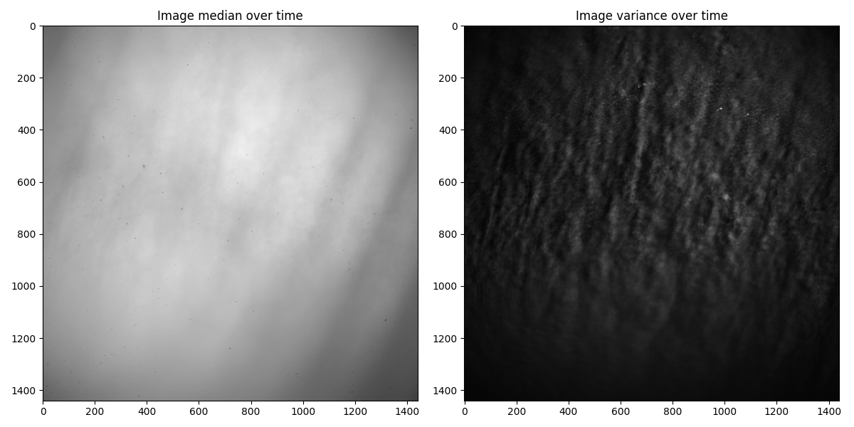
shape: (1440, 1440)

使用局部閾值處理

為了分割污垢點，我們使用閾值處理。我們正在使用的影像光照不均勻，這會導致前景和背景的（絕對）強度發生空間變化。例如，一個區域的平均背景強度可能與另一個（遙遠的）區域不同。因此，跨影像計算不同的閾值（每個區域一個）更為合適。這稱為自適應（或局部）閾值處理，與通常對影像中的所有像素採用單個（全域）閾值的閾值處理程序相反。

當從 filters 模組呼叫 threshold_local 函數時，我們可以變更預設的鄰域大小 (block_size)，即光照變化的典型大小（像素數），以及 offset（移動鄰域的加權平均值）。讓我們嘗試 block_size 的兩個不同值

thresh_1 = ski.filters.threshold_local(image_med, block_size=21, offset=15)
thresh_2 = ski.filters.threshold_local(image_med, block_size=43, offset=15)

mask_1 = image_med < thresh_1
mask_2 = image_med < thresh_2

讓我們定義一個方便的函數來並排顯示兩個圖表，以便我們更容易比較它們

def plot_comparison(plot1, plot2, title1, title2):
    fig, (ax1, ax2) = plt.subplots(ncols=2, figsize=(12, 6), sharex=True, sharey=True)
    ax1.imshow(plot1, cmap='gray')
    ax1.set_title(title1)
    ax2.imshow(plot2, cmap='gray')
    ax2.set_title(title2)


plot_comparison(mask_1, mask_2, "block_size = 21", "block_size = 43")

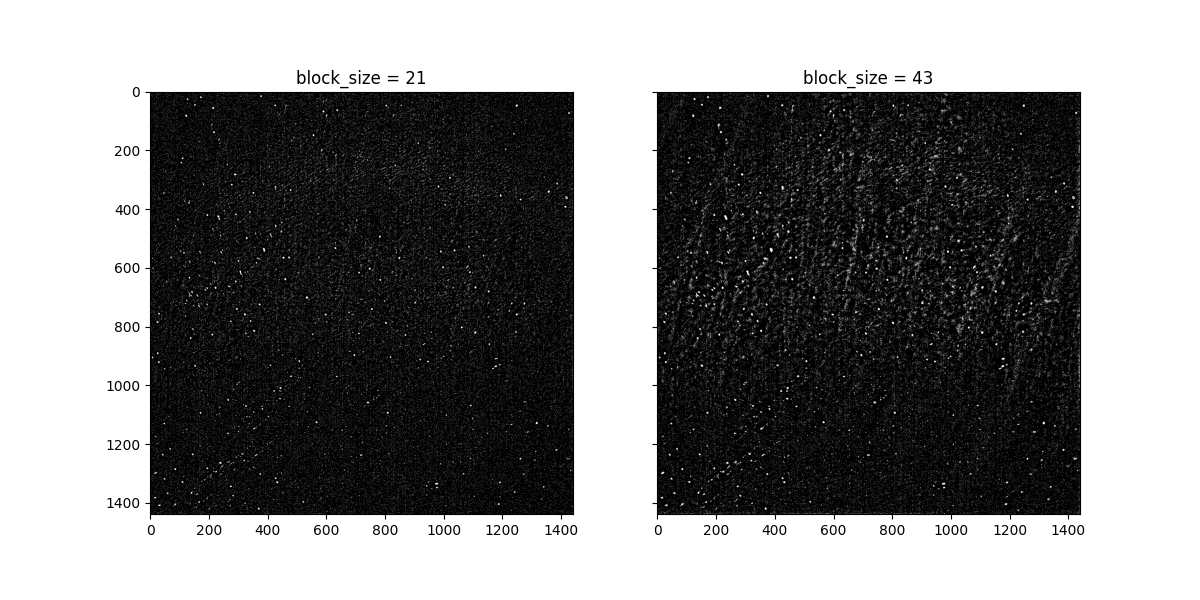
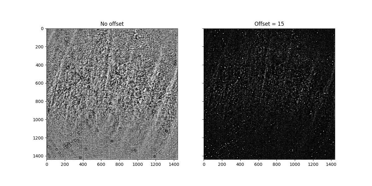
在第二個遮罩中，「污點」似乎更為明顯，也就是使用較大 block_size 值所產生的遮罩。我們注意到，將偏移參數的值從預設的零值增加，會產生更均勻的背景，讓感興趣的物體更明顯地突出。請注意，切換參數值可以讓我們更深入了解所使用的方法，這通常可以使我們更接近期望的結果。

thresh_0 = ski.filters.threshold_local(image_med, block_size=43)

mask_0 = image_med < thresh_0

plot_comparison(mask_0, mask_2, "No offset", "Offset = 15")

移除細微特徵

我們使用形態學濾波器來銳化遮罩並聚焦於污點。兩個基本的形態學運算子是膨脹和侵蝕，其中膨脹（或侵蝕）會將像素設定為結構元素（足跡）定義的鄰域中最亮（或最暗）的值。

在這裡，我們使用 morphology 模組中的 diamond 函式來建立菱形足跡。先進行侵蝕再進行膨脹稱為開運算。首先，我們應用開運算濾波器，以移除小物體和細線，同時保留較大物體的形狀和大小。

footprint = ski.morphology.diamond(3)
mask_open = ski.morphology.opening(mask_2, footprint)
plot_comparison(mask_2, mask_open, "mask before", "after opening")

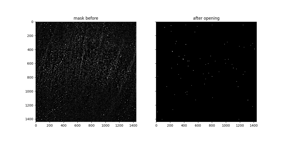
由於「開運算」圖像從侵蝕運算開始，因此小於結構元素的亮區域已被移除。在應用開運算濾波器時，調整足跡參數可讓我們控制移除特徵的細微程度。例如，如果我們在上述內容中使用 footprint = ski.morphology.diamond(1)，我們會看到只有較小的特徵會被濾除，因此在遮罩中保留更多的點。相反地，如果我們使用相同半徑的圓盤狀足跡，也就是 footprint = ski.morphology.disk(3)，則會濾除更多細微的特徵，因為圓盤的面積大於菱形的面積。

接著，我們可以透過應用膨脹濾波器來加寬偵測到的區域。

mask_dilate = ski.morphology.dilation(mask_open, footprint)
plot_comparison(mask_open, mask_dilate, "Before", "After dilation")

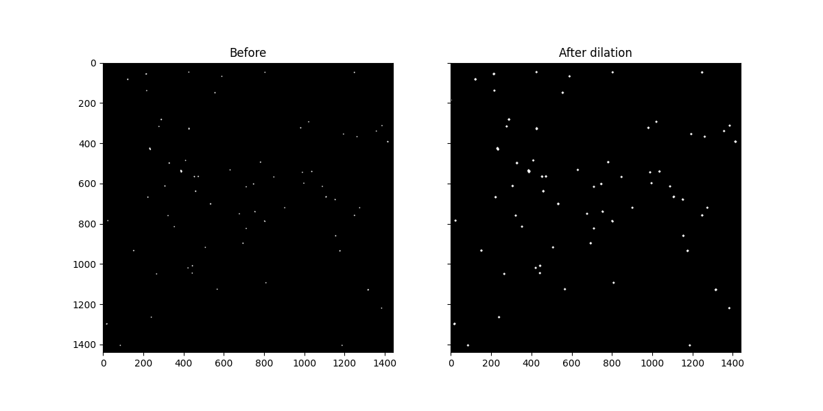
膨脹會擴大亮區域並縮小暗區域。請注意，白點確實是如何加厚的。

分別修復每個影格

現在我們準備好對每個影格應用修復。為此，我們使用 restoration 模組中的 inpaint_biharmonic 函式。它實作基於雙調和方程式的演算法。此函式採用兩個陣列作為輸入：要修復的影像和對應於我們要修復區域的遮罩（具有相同的形狀）。

image_seq_inpainted = np.zeros(image_seq.shape)

for i in range(image_seq.shape[0]):
    image_seq_inpainted[i] = ski.restoration.inpaint_biharmonic(
        image_seq[i], mask_dilate
    )

讓我們視覺化一個已修復的影像，其中污點已被修復。首先，我們找到污點（或遮罩）的輪廓，以便我們可以將它們繪製在修復的影像之上。

contours = ski.measure.find_contours(mask_dilate)

# Gather all (row, column) coordinates of the contours
x = []
y = []
for contour in contours:
    x.append(contour[:, 0])
    y.append(contour[:, 1])
# Note that the following one-liner is equivalent to the above:
# x, y = zip(*((contour[:, 0], contour[:, 1]) for contour in contours))

# Flatten the coordinates
x_flat = np.concatenate(x).ravel().round().astype(int)
y_flat = np.concatenate(y).ravel().round().astype(int)
# Create mask of these contours
contour_mask = np.zeros(mask_dilate.shape, dtype=bool)
contour_mask[x_flat, y_flat] = 1
# Pick one frame
sample_result = image_seq_inpainted[12]
# Normalize it (so intensity values range [0, 1])
sample_result /= sample_result.max()

我們使用 color 模組中的 label2rgb 函式，使用透明度（alpha 參數）將修復的影像與分割的點疊加在一起。

color_contours = ski.color.label2rgb(
    contour_mask, image=sample_result, alpha=0.4, bg_color=(1, 1, 1)
)

fig, ax = plt.subplots(figsize=(6, 6))

ax.imshow(color_contours)
ax.set_title('Segmented spots over restored image')

fig.tight_layout()

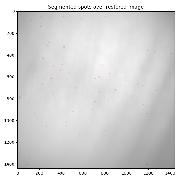
請注意，位於 (x, y) ~ (719, 1237) 的污點很突出；理想情況下，它應該被分割並修復。我們可以發現，在移除細微特徵時，我們在開運算處理步驟中「失去」了它。

plt.show()