使用簡單的影像拼接組裝影像

此範例示範如何在一組剛體運動假設下組裝一組影像。

from matplotlib import pyplot as plt
import numpy as np
from skimage import data, util, transform, feature, measure, filters, metrics


def match_locations(img0, img1, coords0, coords1, radius=5, sigma=3):
    """Match image locations using SSD minimization.

    Areas from `img0` are matched with areas from `img1`. These areas
    are defined as patches located around pixels with Gaussian
    weights.

    Parameters
    ----------
    img0, img1 : 2D array
        Input images.
    coords0 : (2, m) array_like
        Centers of the reference patches in `img0`.
    coords1 : (2, n) array_like
        Centers of the candidate patches in `img1`.
    radius : int
        Radius of the considered patches.
    sigma : float
        Standard deviation of the Gaussian kernel centered over the patches.

    Returns
    -------
    match_coords: (2, m) array
        The points in `coords1` that are the closest corresponding matches to
        those in `coords0` as determined by the (Gaussian weighted) sum of
        squared differences between patches surrounding each point.
    """
    y, x = np.mgrid[-radius : radius + 1, -radius : radius + 1]
    weights = np.exp(-0.5 * (x**2 + y**2) / sigma**2)
    weights /= 2 * np.pi * sigma * sigma

    match_list = []
    for r0, c0 in coords0:
        roi0 = img0[r0 - radius : r0 + radius + 1, c0 - radius : c0 + radius + 1]
        roi1_list = [
            img1[r1 - radius : r1 + radius + 1, c1 - radius : c1 + radius + 1]
            for r1, c1 in coords1
        ]
        # sum of squared differences
        ssd_list = [np.sum(weights * (roi0 - roi1) ** 2) for roi1 in roi1_list]
        match_list.append(coords1[np.argmin(ssd_list)])

    return np.array(match_list)

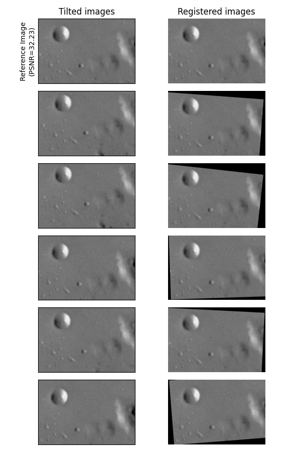
資料產生

在此範例中，我們產生一個稍微傾斜的雜訊影像清單。

img = data.moon()

angle_list = [0, 5, 6, -2, 3, -4]
center_list = [(0, 0), (10, 10), (5, 12), (11, 21), (21, 17), (43, 15)]

img_list = [
    transform.rotate(img, angle=a, center=c)[40:240, 50:350]
    for a, c in zip(angle_list, center_list)
]
ref_img = img_list[0].copy()

img_list = [
    util.random_noise(filters.gaussian(im, sigma=1.1), var=5e-4, rng=seed)
    for seed, im in enumerate(img_list)
]

psnr_ref = metrics.peak_signal_noise_ratio(ref_img, img_list[0])

影像配準

注意

此步驟使用 使用 RANSAC 進行穩健匹配 中描述的方法執行，但您可以根據您的問題應用 影像配準 章節中的任何其他方法。

參考點會在清單中所有影像上偵測。

min_dist = 5
corner_list = [
    feature.corner_peaks(
        feature.corner_harris(img), threshold_rel=0.001, min_distance=min_dist
    )
    for img in img_list
]

在第一張影像中偵測到的 Harris 角點會被選為參考。然後，其他影像上偵測到的點會與參考點進行匹配。

img0 = img_list[0]
coords0 = corner_list[0]
matching_corners = [
    match_locations(img0, img1, coords0, coords1, min_dist)
    for img1, coords1 in zip(img_list, corner_list)
]

一旦所有點都配準到參考點，就可以使用 RANSAC 方法估計穩健的相對仿射變換。

src = np.array(coords0)
trfm_list = [
    measure.ransac(
        (dst, src),
        transform.EuclideanTransform,
        min_samples=3,
        residual_threshold=2,
        max_trials=100,
    )[0].params
    for dst in matching_corners
]

fig, ax_list = plt.subplots(6, 2, figsize=(6, 9), sharex=True, sharey=True)
for idx, (im, trfm, (ax0, ax1)) in enumerate(zip(img_list, trfm_list, ax_list)):
    ax0.imshow(im, cmap="gray", vmin=0, vmax=1)
    ax1.imshow(transform.warp(im, trfm), cmap="gray", vmin=0, vmax=1)

    if idx == 0:
        ax0.set_title("Tilted images")
        ax0.set_ylabel(f"Reference Image\n(PSNR={psnr_ref:.2f})")
        ax1.set_title("Registered images")

    ax0.set(xticklabels=[], yticklabels=[], xticks=[], yticks=[])
    ax1.set_axis_off()

fig.tight_layout()

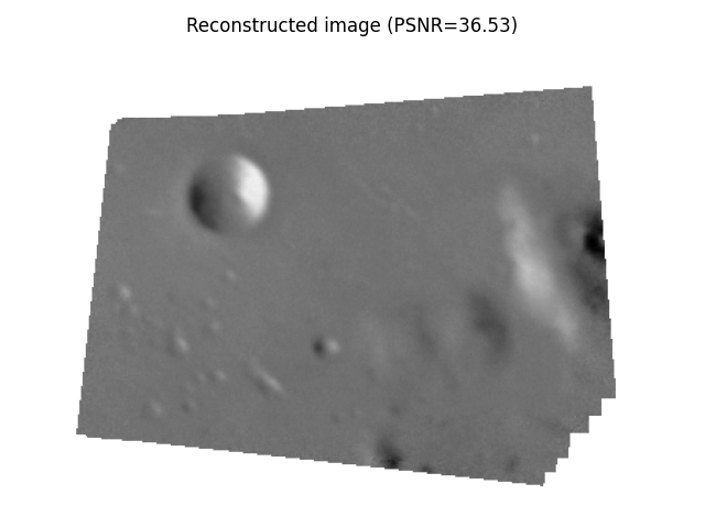
影像組裝

可以使用配準影像相對於參考影像的位置獲得合成影像。為此，我們在參考影像周圍定義一個全域網域，並將其他影像放置在此網域中。

定義一個全域轉換，透過簡單的平移將參考影像移動到全域網域影像中

margin = 50
height, width = img_list[0].shape
out_shape = height + 2 * margin, width + 2 * margin
glob_trfm = np.eye(3)
glob_trfm[:2, 2] = -margin, -margin

最後，透過將全域轉換與相對轉換組合來獲得其他影像在全域網域中的相對位置

global_img_list = [
    transform.warp(
        img, trfm.dot(glob_trfm), output_shape=out_shape, mode="constant", cval=np.nan
    )
    for img, trfm in zip(img_list, trfm_list)
]

all_nan_mask = np.all([np.isnan(img) for img in global_img_list], axis=0)
global_img_list[0][all_nan_mask] = 1.0

composite_img = np.nanmean(global_img_list, 0)
psnr_composite = metrics.peak_signal_noise_ratio(
    ref_img, composite_img[margin : margin + height, margin : margin + width]
)

fig, ax = plt.subplots(1, 1)

ax.imshow(composite_img, cmap="gray", vmin=0, vmax=1)
ax.set_axis_off()
ax.set_title(f"Reconstructed image (PSNR={psnr_composite:.2f})")
fig.tight_layout()

plt.show()