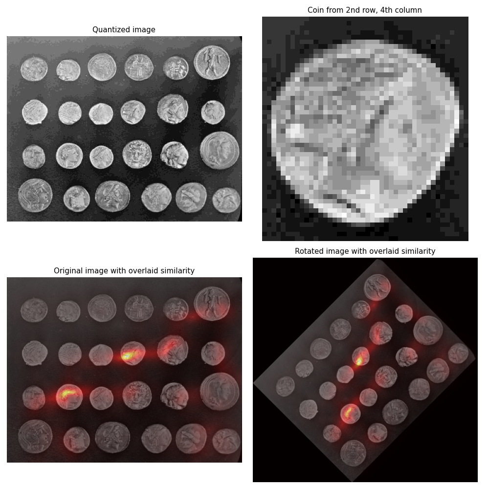
滑動視窗直方圖

直方圖匹配可用於影像中的物件偵測 [1]。此範例從 skimage.data.coins 影像中擷取單個硬幣，並使用直方圖匹配嘗試在原始影像中找到它。

首先，擷取包含目標硬幣的影像的盒狀區域，並計算其灰階值的直方圖。

接著，對於測試影像中的每個像素，計算影像中環繞像素的區域中灰階值的直方圖。 skimage.filters.rank.windowed_histogram 用於此任務，因為它採用基於有效率的滑動視窗的演算法，能夠快速計算這些直方圖 [2]。將影像中每個像素周圍區域的局部直方圖與單個硬幣的直方圖進行比較，計算並顯示相似性度量。

單個硬幣的直方圖是使用 numpy.histogram 在硬幣周圍的盒狀區域計算的，而滑動視窗直方圖是使用略微不同大小的圓盤狀結構元素計算的。這樣做是為了證明即使存在這些差異，該技術仍然可以找到相似性。

為了證明該技術的旋轉不變性，對旋轉 45 度的硬幣影像版本執行相同的測試。

參考文獻

[1]

Porikli, F. “Integral Histogram: A Fast Way to Extract Histograms in Cartesian Spaces” CVPR, 2005. Vol. 1. IEEE, 2005

[2]

S.Perreault and P.Hebert. Median filtering in constant time. Trans. Image Processing, 16(9):2389-2394, 2007.

import numpy as np
import matplotlib
import matplotlib.pyplot as plt

from skimage import data, transform
from skimage.util import img_as_ubyte
from skimage.morphology import disk
from skimage.filters import rank


matplotlib.rcParams['font.size'] = 9


def windowed_histogram_similarity(image, footprint, reference_hist, n_bins):
    # Compute normalized windowed histogram feature vector for each pixel
    px_histograms = rank.windowed_histogram(image, footprint, n_bins=n_bins)

    # Reshape coin histogram to (1,1,N) for broadcast when we want to use it in
    # arithmetic operations with the windowed histograms from the image
    reference_hist = reference_hist.reshape((1, 1) + reference_hist.shape)

    # Compute Chi squared distance metric: sum((X-Y)^2 / (X+Y));
    # a measure of distance between histograms
    X = px_histograms
    Y = reference_hist

    num = (X - Y) ** 2
    denom = X + Y
    denom[denom == 0] = np.inf
    frac = num / denom

    chi_sqr = 0.5 * np.sum(frac, axis=2)

    # Generate a similarity measure. It needs to be low when distance is high
    # and high when distance is low; taking the reciprocal will do this.
    # Chi squared will always be >= 0, add small value to prevent divide by 0.
    similarity = 1 / (chi_sqr + 1.0e-4)

    return similarity


# Load the `skimage.data.coins` image
img = img_as_ubyte(data.coins())

# Quantize to 16 levels of grayscale; this way the output image will have a
# 16-dimensional feature vector per pixel
quantized_img = img // 16

# Select the coin from the 4th column, second row.
# Coordinate ordering: [x1,y1,x2,y2]
coin_coords = [184, 100, 228, 148]  # 44 x 44 region
coin = quantized_img[coin_coords[1] : coin_coords[3], coin_coords[0] : coin_coords[2]]

# Compute coin histogram and normalize
coin_hist, _ = np.histogram(coin.flatten(), bins=16, range=(0, 16))
coin_hist = coin_hist.astype(float) / np.sum(coin_hist)

# Compute a disk shaped mask that will define the shape of our sliding window
# Example coin is ~44px across, so make a disk 61px wide (2 * rad + 1) to be
# big enough for other coins too.
footprint = disk(30)

# Compute the similarity across the complete image
similarity = windowed_histogram_similarity(
    quantized_img, footprint, coin_hist, coin_hist.shape[0]
)

# Now try a rotated image
rotated_img = img_as_ubyte(transform.rotate(img, 45.0, resize=True))
# Quantize to 16 levels as before
quantized_rotated_image = rotated_img // 16
# Similarity on rotated image
rotated_similarity = windowed_histogram_similarity(
    quantized_rotated_image, footprint, coin_hist, coin_hist.shape[0]
)

fig, axes = plt.subplots(nrows=2, ncols=2, figsize=(10, 10))

axes[0, 0].imshow(quantized_img, cmap='gray')
axes[0, 0].set_title('Quantized image')
axes[0, 0].axis('off')

axes[0, 1].imshow(coin, cmap='gray')
axes[0, 1].set_title('Coin from 2nd row, 4th column')
axes[0, 1].axis('off')

axes[1, 0].imshow(img, cmap='gray')
axes[1, 0].imshow(similarity, cmap='hot', alpha=0.5)
axes[1, 0].set_title('Original image with overlaid similarity')
axes[1, 0].axis('off')

axes[1, 1].imshow(rotated_img, cmap='gray')
axes[1, 1].imshow(rotated_similarity, cmap='hot', alpha=0.5)
axes[1, 1].set_title('Rotated image with overlaid similarity')
axes[1, 1].axis('off')

plt.tight_layout()
plt.show()