使用 pandas 探索與視覺化區域屬性

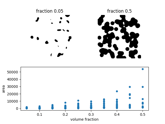
這個玩具範例展示如何計算一系列 10 張影像中每個標記區域的大小。我們使用 2D 影像，然後使用 3D 影像。類斑點區域是合成產生的。隨著體積分數（即斑點覆蓋的像素或體素比例）增加，斑點（區域）的數量減少，而單個區域的大小（面積或體積）可能會越來越大。面積（大小）值以與 pandas 相容的格式提供，這使得資料分析和視覺化更加方便。

除了面積之外，還有許多其他區域屬性可用。

import matplotlib.pyplot as plt
import numpy as np
import pandas as pd
import seaborn as sns

from skimage import data, measure


fractions = np.linspace(0.05, 0.5, 10)

2D 影像

images = [data.binary_blobs(volume_fraction=f) for f in fractions]

labeled_images = [measure.label(image) for image in images]

properties = ['label', 'area']

tables = [
    measure.regionprops_table(image, properties=properties) for image in labeled_images
]
tables = [pd.DataFrame(table) for table in tables]

for fraction, table in zip(fractions, tables):
    table['volume fraction'] = fraction

areas = pd.concat(tables, axis=0)

# Create custom grid of subplots
grid = plt.GridSpec(2, 2)
ax1 = plt.subplot(grid[0, 0])
ax2 = plt.subplot(grid[0, 1])
ax = plt.subplot(grid[1, :])
# Show image with lowest volume fraction
ax1.imshow(images[0], cmap='gray_r')
ax1.set_axis_off()
ax1.set_title(f'fraction {fractions[0]}')
# Show image with highest volume fraction
ax2.imshow(images[-1], cmap='gray_r')
ax2.set_axis_off()
ax2.set_title(f'fraction {fractions[-1]}')
# Plot area vs volume fraction
areas.plot(x='volume fraction', y='area', kind='scatter', ax=ax)
plt.show()

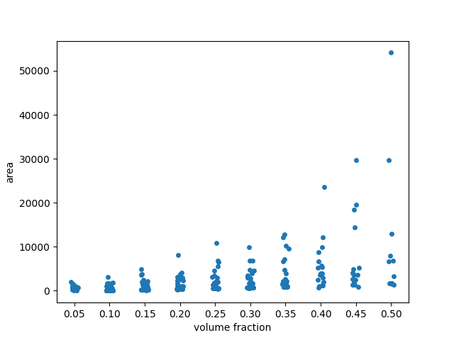
在散佈圖中，許多點似乎在低面積值時重疊。為了更好地了解分佈，我們可能希望為視覺化添加一些「抖動」。為此，我們使用 seaborn.stripplot （來自 seaborn 函式庫，用於統計資料視覺化），並帶有引數 jitter=True。

fig, ax = plt.subplots()
sns.stripplot(x='volume fraction', y='area', data=areas, jitter=True, ax=ax)
# Fix floating point rendering
ax.set_xticklabels([f'{frac:.2f}' for frac in fractions])
plt.show()

/home/runner/work/scikit-image/scikit-image/doc/examples/segmentation/plot_regionprops_table.py:75: UserWarning:

set_ticklabels() should only be used with a fixed number of ticks, i.e. after set_ticks() or using a FixedLocator.

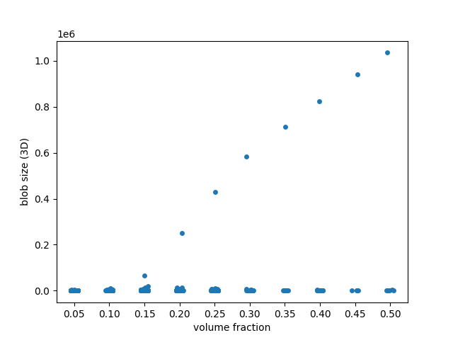
3D 影像

在 3D 中進行相同的分析，我們發現了一個更戲劇性的行為：當體積分數超過 ~0.25 時，斑點會合併成單個巨大的塊。這對應於統計物理學和圖論中的滲濾閾值。

images = [data.binary_blobs(length=128, n_dim=3, volume_fraction=f) for f in fractions]

labeled_images = [measure.label(image) for image in images]

properties = ['label', 'area']

tables = [
    measure.regionprops_table(image, properties=properties) for image in labeled_images
]
tables = [pd.DataFrame(table) for table in tables]

for fraction, table in zip(fractions, tables):
    table['volume fraction'] = fraction

blob_volumes = pd.concat(tables, axis=0)

fig, ax = plt.subplots()
sns.stripplot(x='volume fraction', y='area', data=blob_volumes, jitter=True, ax=ax)
ax.set_ylabel('blob size (3D)')
# Fix floating point rendering
ax.set_xticklabels([f'{frac:.2f}' for frac in fractions])
plt.show()

/home/runner/work/scikit-image/scikit-image/doc/examples/segmentation/plot_regionprops_table.py:107: UserWarning:

set_ticklabels() should only be used with a fixed number of ticks, i.e. after set_ticks() or using a FixedLocator.