測量核膜的螢光強度

此範例重現了生物影像數據分析中一個完善的工作流程，用於測量定位在核膜上的螢光強度，在細胞影像的時間序列（每個影像具有兩個通道和兩個空間維度）中，顯示了蛋白質從細胞質區域重新定位到核膜的過程。這個生物應用程式最初由 Andrea Boni 及其合作者在 [1] 中提出；它被 Kota Miura 在教科書 [2] 以及其他著作 ([3], [4]) 中使用。換句話說，我們將此工作流程從 ImageJ Macro 移植到 Python 與 scikit-image。

[1]

Boni A, Politi AZ, Strnad P, Xiang W, Hossain MJ, Ellenberg J (2015) “Live imaging and modeling of inner nuclear membrane targeting reveals its molecular requirements in mammalian cells” J Cell Biol 209(5):705–720. ISSN: 0021-9525. DOI:10.1083/jcb.201409133

[2]

Miura K (2020) “Measurements of Intensity Dynamics at the Periphery of the Nucleus” in: Miura K, Sladoje N (eds) Bioimage Data Analysis Workflows. Learning Materials in Biosciences. Springer, Cham. DOI:10.1007/978-3-030-22386-1_2

[3]

Klemm A (2020) “ImageJ/Fiji Macro Language” NEUBIAS Academy Online Course: https://www.youtube.com/watch?v=o8tfkdcd3DA

[4]

Vorkel D and Haase R (2020) “GPU-accelerating ImageJ Macro image processing workflows using CLIJ” https://arxiv.org/abs/2008.11799

import matplotlib.pyplot as plt
import numpy as np
import plotly.io
import plotly.express as px
from scipy import ndimage as ndi

from skimage import filters, measure, morphology, segmentation
from skimage.data import protein_transport

我們先從單個細胞/細胞核開始構建工作流程。

image_sequence = protein_transport()

print(f'shape: {image_sequence.shape}')

shape: (15, 2, 180, 183)

資料集是一個 2D 影像堆疊，包含 15 個影格（時間點）和 2 個通道。

vmin, vmax = 0, image_sequence.max()

fig = px.imshow(
    image_sequence,
    facet_col=1,
    animation_frame=0,
    zmin=vmin,
    zmax=vmax,
    binary_string=True,
    labels={'animation_frame': 'time point', 'facet_col': 'channel'},
)
plotly.io.show(fig)

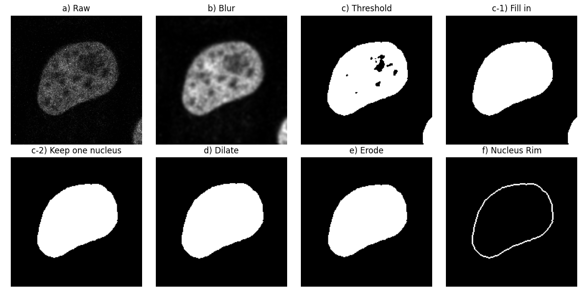
首先，讓我們考慮第一個影像的第一個通道（下圖中的步驟 a)）。

image_t_0_channel_0 = image_sequence[0, 0, :, :]

分割細胞核邊緣

讓我們將高斯低通濾波器應用於此影像以使其平滑（步驟 b)）。接下來，我們分割細胞核，使用 Otsu 的方法找到背景和前景之間的閾值：我們得到一個二元影像（步驟 c)）。然後，我們填補物件中的孔洞（步驟 c-1)）。

smooth = filters.gaussian(image_t_0_channel_0, sigma=1.5)

thresh_value = filters.threshold_otsu(smooth)
thresh = smooth > thresh_value

fill = ndi.binary_fill_holes(thresh)

依照原始工作流程，讓我們移除接觸影像邊界的物件（步驟 c-2)）。在這裡，我們可以看見另一個細胞核的一部分接觸到右下角。

clear = segmentation.clear_border(fill)
clear.dtype

dtype('bool')

我們計算此二元影像的形態膨脹（步驟 d)）和形態侵蝕（步驟 e)）。

dilate = morphology.binary_dilation(clear)

erode = morphology.binary_erosion(clear)

最後，我們從膨脹中減去侵蝕以得到細胞核邊緣（步驟 f)）。這相當於選擇 dilate 中但不屬於 erode 的像素

mask = np.logical_and(dilate, ~erode)

讓我們在子圖序列中視覺化這些處理步驟。

fig, ax = plt.subplots(2, 4, figsize=(12, 6), sharey=True)

ax[0, 0].imshow(image_t_0_channel_0, cmap=plt.cm.gray)
ax[0, 0].set_title('a) Raw')

ax[0, 1].imshow(smooth, cmap=plt.cm.gray)
ax[0, 1].set_title('b) Blur')

ax[0, 2].imshow(thresh, cmap=plt.cm.gray)
ax[0, 2].set_title('c) Threshold')

ax[0, 3].imshow(fill, cmap=plt.cm.gray)
ax[0, 3].set_title('c-1) Fill in')

ax[1, 0].imshow(clear, cmap=plt.cm.gray)
ax[1, 0].set_title('c-2) Keep one nucleus')

ax[1, 1].imshow(dilate, cmap=plt.cm.gray)
ax[1, 1].set_title('d) Dilate')

ax[1, 2].imshow(erode, cmap=plt.cm.gray)
ax[1, 2].set_title('e) Erode')

ax[1, 3].imshow(mask, cmap=plt.cm.gray)
ax[1, 3].set_title('f) Nucleus Rim')

for a in ax.ravel():
    a.set_axis_off()

fig.tight_layout()

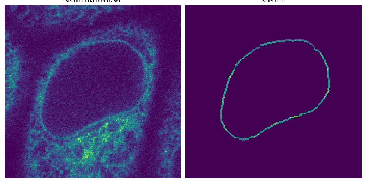
將分割的邊緣作為遮罩應用

現在我們已經分割了第一個通道中的核膜，我們將其用作遮罩來測量第二個通道中的強度。

image_t_0_channel_1 = image_sequence[0, 1, :, :]
selection = np.where(mask, image_t_0_channel_1, 0)

fig, (ax0, ax1) = plt.subplots(1, 2, figsize=(12, 6), sharey=True)

ax0.imshow(image_t_0_channel_1)
ax0.set_title('Second channel (raw)')
ax0.set_axis_off()

ax1.imshow(selection)
ax1.set_title('Selection')
ax1.set_axis_off()

fig.tight_layout()

測量總強度

平均強度可以很容易地作為標記圖像中的區域屬性取得。

props = measure.regionprops_table(
    mask.astype(np.uint8),
    intensity_image=image_t_0_channel_1,
    properties=('label', 'area', 'intensity_mean'),
)

我們可能需要檢查總強度的值

selection.sum()

np.uint64(28350)

是否可以從以下方式還原

props['area'] * props['intensity_mean']

array([28350.])

處理整個影像序列

我們並非針對每個時間點迭代工作流程，而是直接處理多維數據集（除了閾值處理步驟）。事實上，大多數 scikit-image 函數都支援 n 維圖像。

n_z = image_sequence.shape[0]  # number of frames

smooth_seq = filters.gaussian(image_sequence[:, 0, :, :], sigma=(0, 1.5, 1.5))
thresh_values = [filters.threshold_otsu(s) for s in smooth_seq[:]]
thresh_seq = [smooth_seq[k, ...] > val for k, val in enumerate(thresh_values)]

或者，我們可以計算 thresh_values，而無需使用列表推導式，方法是將 smooth_seq 重塑為 2D（其中第一維仍然對應於時間點，但第二維和最後一維現在包含所有像素值），並沿其第二軸對影像序列應用閾值處理函數

thresh_values = np.apply_along_axis(filters.threshold_otsu,
                                    axis=1,
                                    arr=smooth_seq.reshape(n_z, -1))

我們使用以下扁平結構元素進行形態學計算（np.newaxis 用於在時間軸前添加大小為 1 的軸）

footprint = ndi.generate_binary_structure(2, 1)[np.newaxis, ...]
footprint

array([[[False,  True, False],
        [ True,  True,  True],
        [False,  True, False]]])

這樣一來，每個影格都會被獨立處理（來自連續影格的像素永遠不會是空間上的相鄰像素）。

fill_seq = ndi.binary_fill_holes(thresh_seq, structure=footprint)

當清除接觸圖像邊界的物件時，我們希望確保底部（第一個）和頂部（最後一個）影格不被視為邊界。在這種情況下，唯一相關的邊界是最大 (x, y) 值處的邊緣。通過運行以下程式碼，可以在 3D 中看到這一點

import plotly.graph_objects as go

sample = fill_seq
(n_Z, n_Y, n_X) = sample.shape
Z, Y, X = np.mgrid[:n_Z, :n_Y, :n_X]

fig = go.Figure(
    data=go.Volume(
        x=X.flatten(),
        y=Y.flatten(),
        z=Z.flatten(),
        value=sample.flatten(),
        opacity=0.5,
        slices_z=dict(show=True, locations=[n_z // 2])
    )
)
fig.show()

border_mask = np.ones_like(fill_seq)
border_mask[n_z // 2, -1, -1] = False
clear_seq = segmentation.clear_border(fill_seq, mask=border_mask)

dilate_seq = morphology.binary_dilation(clear_seq, footprint=footprint)
erode_seq = morphology.binary_erosion(clear_seq, footprint=footprint)
mask_sequence = np.logical_and(dilate_seq, ~erode_seq)

讓我們為每個遮罩（對應於每個時間點）賦予不同的標籤，從 1 到 15。我們使用 np.min_scalar_type 來確定表示時間點數量所需最小尺寸的整數 dtype

label_dtype = np.min_scalar_type(n_z)
mask_sequence = mask_sequence.astype(label_dtype)
labels = np.arange(1, n_z + 1, dtype=label_dtype)
mask_sequence *= labels[:, np.newaxis, np.newaxis]

讓我們計算所有這些標記區域感興趣的區域屬性。

props = measure.regionprops_table(
    mask_sequence,
    intensity_image=image_sequence[:, 1, :, :],
    properties=('label', 'area', 'intensity_mean'),
)
np.testing.assert_array_equal(props['label'], np.arange(n_z) + 1)

fluorescence_change = [
    props['area'][i] * props['intensity_mean'][i] for i in range(n_z)
]

fluorescence_change /= fluorescence_change[0]  # normalization

fig, ax = plt.subplots()
ax.plot(fluorescence_change, 'rs')
ax.grid()
ax.set_xlabel('Time point')
ax.set_ylabel('Normalized total intensity')
ax.set_title('Change in fluorescence intensity at the nuclear envelope')
fig.tight_layout()

plt.show()

令人欣慰的是，我們找到了預期的結果：在最初的五個時間點，核膜的總螢光強度增加了 1.3 倍，然後大致變得恆定。