共定位指標

在此範例中，我們示範使用不同的指標來評估兩個不同影像通道的共定位。

共定位可以分為兩個不同的概念：1. 共現性：有多少比例的物質定位到特定區域？2. 相關性：兩種物質之間的強度關係是什麼？

共現性：亞細胞定位

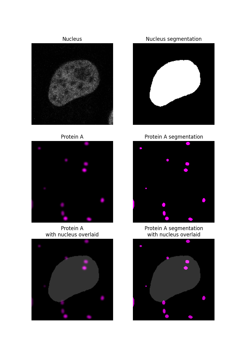
想像一下，我們試圖確定蛋白質的亞細胞定位 - 與對照組相比，它是否更多地定位在細胞核或細胞質中？

我們先分割樣本影像的細胞核，如另一個範例所述，並假設不在細胞核中的任何物質都在細胞質中。「蛋白質 A」將被模擬為斑點並分割。

import matplotlib.pyplot as plt
import numpy as np
from matplotlib.colors import LinearSegmentedColormap
from scipy import ndimage as ndi
from skimage import data, filters, measure, segmentation

rng = np.random.default_rng()

# segment nucleus
nucleus = data.protein_transport()[0, 0, :, :180]
smooth = filters.gaussian(nucleus, sigma=1.5)
thresh = smooth > filters.threshold_otsu(smooth)
fill = ndi.binary_fill_holes(thresh)
nucleus_seg = segmentation.clear_border(fill)

# protein blobs of varying intensity
proteinA = np.zeros_like(nucleus, dtype="float64")
proteinA_seg = np.zeros_like(nucleus, dtype="float64")

for blob_seed in range(10):
    blobs = data.binary_blobs(
        180, blob_size_fraction=0.5, volume_fraction=(50 / (180**2)), rng=blob_seed
    )
    blobs_image = filters.gaussian(blobs, sigma=1.5) * rng.integers(50, 256)
    proteinA += blobs_image
    proteinA_seg += blobs

# plot data
fig, ax = plt.subplots(3, 2, figsize=(8, 12), sharey=True)
ax[0, 0].imshow(nucleus, cmap=plt.cm.gray)
ax[0, 0].set_title('Nucleus')

ax[0, 1].imshow(nucleus_seg, cmap=plt.cm.gray)
ax[0, 1].set_title('Nucleus segmentation')

black_magenta = LinearSegmentedColormap.from_list("", ["black", "magenta"])
ax[1, 0].imshow(proteinA, cmap=black_magenta)
ax[1, 0].set_title('Protein A')

ax[1, 1].imshow(proteinA_seg, cmap=black_magenta)
ax[1, 1].set_title('Protein A segmentation')

ax[2, 0].imshow(proteinA, cmap=black_magenta)
ax[2, 0].imshow(nucleus_seg, cmap=plt.cm.gray, alpha=0.2)
ax[2, 0].set_title('Protein A\nwith nucleus overlaid')

ax[2, 1].imshow(proteinA_seg, cmap=black_magenta)
ax[2, 1].imshow(nucleus_seg, cmap=plt.cm.gray, alpha=0.2)
ax[2, 1].set_title('Protein A segmentation\nwith nucleus overlaid')

for a in ax.ravel():
    a.set_axis_off()

交集係數

在分割細胞核和目標蛋白質後，我們可以確定蛋白質 A 分割與細胞核分割重疊的比例。

measure.intersection_coeff(proteinA_seg, nucleus_seg)

0.22

曼德斯共定位係數 (MCC)

重疊係數假設蛋白質分割的面積對應於該蛋白質的濃度 - 較大的面積表示更多的蛋白質。由於影像的解析度通常太小而無法分辨出個別的蛋白質，它們可以在一個像素內聚集在一起，使該像素的強度更亮。因此，為了更好地捕捉蛋白質濃度，我們可能會選擇確定蛋白質通道的強度有多少比例在細胞核內。此指標稱為曼德斯共定位係數。

在此影像中，雖然細胞核內有很多蛋白質 A 的斑點，但與細胞核外的一些斑點相比，它們很暗淡，因此 MCC 比重疊係數低得多。

measure.manders_coloc_coeff(proteinA, nucleus_seg)

np.float64(0.2566709686373243)

選擇共現性指標後，我們可以將相同的流程應用於對照影像。如果沒有可用的對照影像，可以使用 Costes 方法將原始影像的 MCC 值與隨機打亂影像的 MCC 值進行比較。有關此方法的資訊在[1]中給出。

[1]

J. S. Aaron, A. B. Taylor and T.-L. Chew, Image co-localization – co-occurrence versus correlation. J Cell Sci 1 February 2018 131 (3): jcs211847. doi: https://doi.org/10.1242/jcs.211847

相關性：兩種蛋白質的關聯

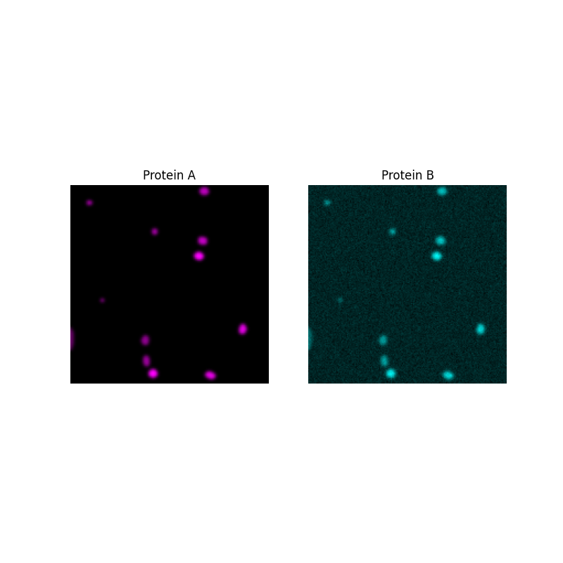
現在，假設我們想知道兩種蛋白質的關聯程度有多密切。

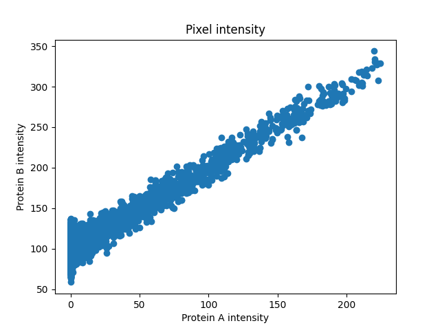
首先，我們將產生蛋白質 B 並繪製每個像素中兩種蛋白質的強度，以查看它們之間的關係。

# generating protein B data that is correlated to protein A for demo
proteinB = proteinA + rng.normal(loc=100, scale=10, size=proteinA.shape)

# plot images
fig, ax = plt.subplots(1, 2, figsize=(8, 8), sharey=True)

ax[0].imshow(proteinA, cmap=black_magenta)
ax[0].set_title('Protein A')

black_cyan = LinearSegmentedColormap.from_list("", ["black", "cyan"])
ax[1].imshow(proteinB, cmap=black_cyan)
ax[1].set_title('Protein B')

for a in ax.ravel():
    a.set_axis_off()

# plot pixel intensity scatter
fig, ax = plt.subplots()
ax.scatter(proteinA, proteinB)
ax.set_title('Pixel intensity')
ax.set_xlabel('Protein A intensity')
ax.set_ylabel('Protein B intensity')

• 
• 

Text(38.347222222222214, 0.5, 'Protein B intensity')

強度看起來呈線性相關，因此皮爾森相關係數可以很好地衡量關聯的強度。

pcc, pval = measure.pearson_corr_coeff(proteinA, proteinB)
print(f"PCC: {pcc:0.3g}, p-val: {pval:0.3g}")

PCC: 0.857, p-val: 0

有時強度是相關的，但不是線性相關。在這種情況下，像 Spearman's 這樣的基於等級的相關係數可能會更準確地衡量非線性關係。

plt.show()