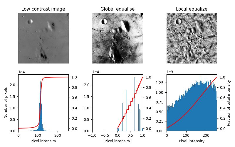
局部直方圖均衡化

此範例使用一種稱為局部直方圖均衡化的方法來增強低對比度的影像，該方法會展開影像中最頻繁的強度值。

對於每個像素鄰域，均衡化的影像[1]具有大致線性的累積分布函數。

局部版本的直方圖均衡化[2]強調了每個局部灰階變化。

這些演算法可以用於 2D 和 3D 影像。

參考文獻

[1]

https://en.wikipedia.org/wiki/Histogram_equalization

[2]

https://en.wikipedia.org/wiki/Adaptive_histogram_equalization

import numpy as np
import matplotlib
import matplotlib.pyplot as plt

from skimage import data
from skimage.util.dtype import dtype_range
from skimage.util import img_as_ubyte
from skimage import exposure
from skimage.morphology import disk
from skimage.morphology import ball
from skimage.filters import rank


matplotlib.rcParams['font.size'] = 9


def plot_img_and_hist(image, axes, bins=256):
    """Plot an image along with its histogram and cumulative histogram."""
    ax_img, ax_hist = axes
    ax_cdf = ax_hist.twinx()

    # Display image
    ax_img.imshow(image, cmap=plt.cm.gray)
    ax_img.set_axis_off()

    # Display histogram
    ax_hist.hist(image.ravel(), bins=bins)
    ax_hist.ticklabel_format(axis='y', style='scientific', scilimits=(0, 0))
    ax_hist.set_xlabel('Pixel intensity')

    xmin, xmax = dtype_range[image.dtype.type]
    ax_hist.set_xlim(xmin, xmax)

    # Display cumulative distribution
    img_cdf, bins = exposure.cumulative_distribution(image, bins)
    ax_cdf.plot(bins, img_cdf, 'r')

    return ax_img, ax_hist, ax_cdf


# Load an example image
img = img_as_ubyte(data.moon())

# Global equalize
img_rescale = exposure.equalize_hist(img)

# Equalization
footprint = disk(30)
img_eq = rank.equalize(img, footprint=footprint)


# Display results
fig = plt.figure(figsize=(8, 5))
axes = np.zeros((2, 3), dtype=object)
axes[0, 0] = plt.subplot(2, 3, 1)
axes[0, 1] = plt.subplot(2, 3, 2, sharex=axes[0, 0], sharey=axes[0, 0])
axes[0, 2] = plt.subplot(2, 3, 3, sharex=axes[0, 0], sharey=axes[0, 0])
axes[1, 0] = plt.subplot(2, 3, 4)
axes[1, 1] = plt.subplot(2, 3, 5)
axes[1, 2] = plt.subplot(2, 3, 6)

ax_img, ax_hist, ax_cdf = plot_img_and_hist(img, axes[:, 0])
ax_img.set_title('Low contrast image')
ax_hist.set_ylabel('Number of pixels')

ax_img, ax_hist, ax_cdf = plot_img_and_hist(img_rescale, axes[:, 1])
ax_img.set_title('Global equalise')

ax_img, ax_hist, ax_cdf = plot_img_and_hist(img_eq, axes[:, 2])
ax_img.set_title('Local equalize')
ax_cdf.set_ylabel('Fraction of total intensity')


# prevent overlap of y-axis labels
fig.tight_layout()

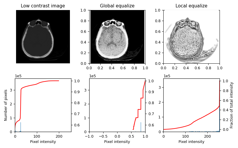
3D 均衡化

3D 體積也可以用類似的方式進行均衡化。這裡的直方圖是從整個 3D 影像收集的，但為了視覺檢查，只顯示一個切片。

matplotlib.rcParams['font.size'] = 9


def plot_img_and_hist(image, axes, bins=256):
    """Plot an image along with its histogram and cumulative histogram."""
    ax_img, ax_hist = axes
    ax_cdf = ax_hist.twinx()

    # Display Slice of Image
    ax_img.imshow(image[0], cmap=plt.cm.gray)
    ax_img.set_axis_off()

    # Display histogram
    ax_hist.hist(image.ravel(), bins=bins)
    ax_hist.ticklabel_format(axis='y', style='scientific', scilimits=(0, 0))
    ax_hist.set_xlabel('Pixel intensity')

    xmin, xmax = dtype_range[image.dtype.type]
    ax_hist.set_xlim(xmin, xmax)

    # Display cumulative distribution
    img_cdf, bins = exposure.cumulative_distribution(image, bins)
    ax_cdf.plot(bins, img_cdf, 'r')

    return ax_img, ax_hist, ax_cdf


# Load an example image
img = img_as_ubyte(data.brain())

# Global equalization
img_rescale = exposure.equalize_hist(img)

# Local equalization
neighborhood = ball(3)
img_eq = rank.equalize(img, footprint=neighborhood)

# Display results
fig, axes = plt.subplots(2, 3, figsize=(8, 5))
axes[0, 1] = plt.subplot(2, 3, 2, sharex=axes[0, 0], sharey=axes[0, 0])
axes[0, 2] = plt.subplot(2, 3, 3, sharex=axes[0, 0], sharey=axes[0, 0])

ax_img, ax_hist, ax_cdf = plot_img_and_hist(img, axes[:, 0])
ax_img.set_title('Low contrast image')
ax_hist.set_ylabel('Number of pixels')

ax_img, ax_hist, ax_cdf = plot_img_and_hist(img_rescale, axes[:, 1])
ax_img.set_title('Global equalize')

ax_img, ax_hist, ax_cdf = plot_img_and_hist(img_eq, axes[:, 2])
ax_img.set_title('Local equalize')
ax_cdf.set_ylabel('Fraction of total intensity')


# prevent overlap of y-axis labels
fig.tight_layout()
plt.show()