Li 閾值處理

在 1993 年，Li 和 Lee 提出了一個新的標準，用於尋找「最佳」閾值以區分影像的背景和前景 [1]。 他們提出，最小化前景和前景平均值之間，以及背景和背景平均值之間的交叉熵，將在大多數情況下給出最佳閾值。

然而，直到 1998 年，找到這個閾值的方法是嘗試所有可能的閾值，然後選擇交叉熵最小的那個。在那時，Li 和 Tam 實施了一種新的迭代方法，透過使用交叉熵的斜率來更快地找到最佳點 [2]。 這是在 scikit-image 的 skimage.filters.threshold_li() 中實作的方法。

在這裡，我們展示了交叉熵及其透過 Li 的迭代方法進行的最佳化。 請注意，我們正在使用私有函數 _cross_entropy，它不應在生產程式碼中使用，因為它可能會變更。

[1]

Li C.H. 和 Lee C.K. (1993) “最小交叉熵閾值處理” 模式識別，26(4): 617-625 DOI:10.1016/0031-3203(93)90115-D

[2]

Li C.H. 和 Tam P.K.S. (1998) “最小交叉熵閾值處理的迭代演算法” 模式識別快報，18(8): 771-776 DOI:10.1016/S0167-8655(98)00057-9

import numpy as np
import matplotlib.pyplot as plt
from skimage import data
from skimage import filters
from skimage.filters.thresholding import _cross_entropy

cell = data.cell()
camera = data.camera()

首先，讓我們繪製 skimage.data.camera() 影像在所有可能閾值下的交叉熵。

thresholds = np.arange(np.min(camera) + 1.5, np.max(camera) - 1.5)
entropies = [_cross_entropy(camera, t) for t in thresholds]

optimal_camera_threshold = thresholds[np.argmin(entropies)]

fig, ax = plt.subplots(1, 3, figsize=(8, 3))

ax[0].imshow(camera, cmap='gray')
ax[0].set_title('image')
ax[0].set_axis_off()

ax[1].imshow(camera > optimal_camera_threshold, cmap='gray')
ax[1].set_title('thresholded')
ax[1].set_axis_off()

ax[2].plot(thresholds, entropies)
ax[2].set_xlabel('thresholds')
ax[2].set_ylabel('cross-entropy')
ax[2].vlines(
    optimal_camera_threshold,
    ymin=np.min(entropies) - 0.05 * np.ptp(entropies),
    ymax=np.max(entropies) - 0.05 * np.ptp(entropies),
)
ax[2].set_title('optimal threshold')

fig.tight_layout()

print('The brute force optimal threshold is:', optimal_camera_threshold)
print('The computed optimal threshold is:', filters.threshold_li(camera))

plt.show()

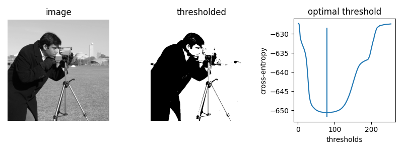
The brute force optimal threshold is: 78.5
The computed optimal threshold is: 78.91288426606151

接下來，讓我們使用 threshold_li 的 iter_callback 功能來檢查最佳化過程的發生情況。

iter_thresholds = []

optimal_threshold = filters.threshold_li(camera, iter_callback=iter_thresholds.append)
iter_entropies = [_cross_entropy(camera, t) for t in iter_thresholds]

print('Only', len(iter_thresholds), 'thresholds examined.')

fig, ax = plt.subplots()

ax.plot(thresholds, entropies, label='all threshold entropies')
ax.plot(iter_thresholds, iter_entropies, label='optimization path')
ax.scatter(iter_thresholds, iter_entropies, c='C1')
ax.legend(loc='upper right')

plt.show()

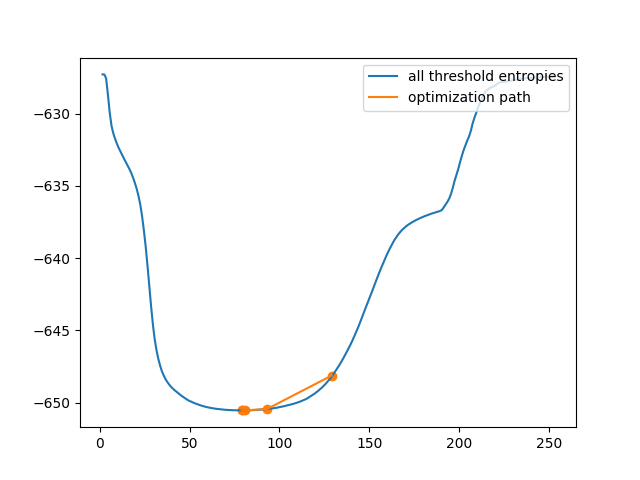
Only 5 thresholds examined.

這顯然比暴力破解方法有效得多。 然而，在某些影像中，交叉熵不是凸的，這意味著只有一個最佳值。 在這種情況下，梯度下降可能會產生非最佳的閾值。 在這個範例中，我們看到不好的最佳化初始猜測會導致不良的閾值選擇。

iter_thresholds2 = []

opt_threshold2 = filters.threshold_li(
    cell, initial_guess=64, iter_callback=iter_thresholds2.append
)

thresholds2 = np.arange(np.min(cell) + 1.5, np.max(cell) - 1.5)
entropies2 = [_cross_entropy(cell, t) for t in thresholds]
iter_entropies2 = [_cross_entropy(cell, t) for t in iter_thresholds2]

fig, ax = plt.subplots(1, 3, figsize=(8, 3))

ax[0].imshow(cell, cmap='magma')
ax[0].set_title('image')
ax[0].set_axis_off()

ax[1].imshow(cell > opt_threshold2, cmap='gray')
ax[1].set_title('thresholded')
ax[1].set_axis_off()

ax[2].plot(thresholds2, entropies2, label='all threshold entropies')
ax[2].plot(iter_thresholds2, iter_entropies2, label='optimization path')
ax[2].scatter(iter_thresholds2, iter_entropies2, c='C1')
ax[2].legend(loc='upper right')

plt.show()

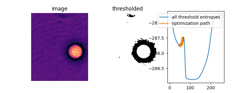
在這個影像中，令人驚訝的是，預設初始猜測，即影像平均值，實際上正好位於目標函數兩個「谷」之間的峰頂。 如果不提供初始猜測，Li 的閾值處理方法根本不會執行任何操作！

iter_thresholds3 = []

opt_threshold3 = filters.threshold_li(cell, iter_callback=iter_thresholds3.append)

iter_entropies3 = [_cross_entropy(cell, t) for t in iter_thresholds3]

fig, ax = plt.subplots(1, 3, figsize=(8, 3))

ax[0].imshow(cell, cmap='magma')
ax[0].set_title('image')
ax[0].set_axis_off()

ax[1].imshow(cell > opt_threshold3, cmap='gray')
ax[1].set_title('thresholded')
ax[1].set_axis_off()

ax[2].plot(thresholds2, entropies2, label='all threshold entropies')
ax[2].plot(iter_thresholds3, iter_entropies3, label='optimization path')
ax[2].scatter(iter_thresholds3, iter_entropies3, c='C1')
ax[2].legend(loc='upper right')

plt.show()

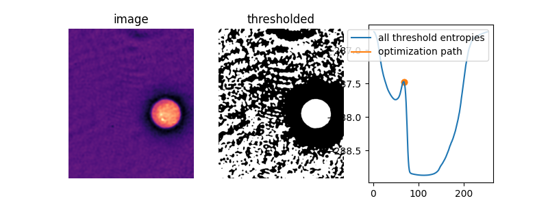
為了了解發生了什麼，讓我們定義一個函數 li_gradient，它會複製 Li 方法的內部迴圈，並返回從目前閾值到下一個閾值的變更。 當這個梯度為 0 時，我們處於所謂的靜止點，Li 會返回這個值。 當它是負數時，下一個閾值猜測將較低，而當它是正數時，下一個猜測將較高。

在下面的圖中，我們顯示了當初始猜測位於熵峰值的右側時的交叉熵和 Li 更新路徑。 我們覆蓋了閾值更新梯度，用 threshold_li 標記 0 梯度線和預設初始猜測。

def li_gradient(image, t):
    """Find the threshold update at a given threshold."""
    foreground = image > t
    mean_fore = np.mean(image[foreground])
    mean_back = np.mean(image[~foreground])
    t_next = (mean_back - mean_fore) / (np.log(mean_back) - np.log(mean_fore))
    dt = t_next - t
    return dt


iter_thresholds4 = []
opt_threshold4 = filters.threshold_li(
    cell, initial_guess=68, iter_callback=iter_thresholds4.append
)
iter_entropies4 = [_cross_entropy(cell, t) for t in iter_thresholds4]
print(len(iter_thresholds4), 'examined, optimum:', opt_threshold4)

gradients = [li_gradient(cell, t) for t in thresholds2]

fig, ax1 = plt.subplots()
ax1.plot(thresholds2, entropies2)
ax1.plot(iter_thresholds4, iter_entropies4)
ax1.scatter(iter_thresholds4, iter_entropies4, c='C1')
ax1.set_xlabel('threshold')
ax1.set_ylabel('cross entropy', color='C0')
ax1.tick_params(axis='y', labelcolor='C0')

ax2 = ax1.twinx()
ax2.plot(thresholds2, gradients, c='C3')
ax2.hlines(
    [0], xmin=thresholds2[0], xmax=thresholds2[-1], colors='gray', linestyles='dashed'
)
ax2.vlines(
    np.mean(cell),
    ymin=np.min(gradients),
    ymax=np.max(gradients),
    colors='gray',
    linestyles='dashed',
)
ax2.set_ylabel(r'$\Delta$(threshold)', color='C3')
ax2.tick_params(axis='y', labelcolor='C3')

fig.tight_layout()

plt.show()

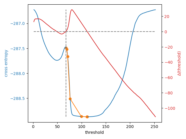
8 examined, optimum: 111.68876119648344

除了允許使用者提供一個數字作為初始猜測外，skimage.filters.threshold_li() 可以接收一個函數，該函數可以像預設情況下的 numpy.mean() 一樣，根據影像強度進行猜測。 當需要處理許多不同範圍的影像時，這可能是一個不錯的選擇。

def quantile_95(image):
    # you can use np.quantile(image, 0.95) if you have NumPy>=1.15
    return np.percentile(image, 95)


iter_thresholds5 = []
opt_threshold5 = filters.threshold_li(
    cell, initial_guess=quantile_95, iter_callback=iter_thresholds5.append
)
iter_entropies5 = [_cross_entropy(cell, t) for t in iter_thresholds5]
print(len(iter_thresholds5), 'examined, optimum:', opt_threshold5)

fig, ax1 = plt.subplots()
ax1.plot(thresholds2, entropies2)
ax1.plot(iter_thresholds5, iter_entropies5)
ax1.scatter(iter_thresholds5, iter_entropies5, c='C1')
ax1.set_xlabel('threshold')
ax1.set_ylabel('cross entropy', color='C0')
ax1.tick_params(axis='y', labelcolor='C0')

plt.show()

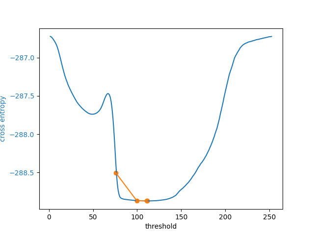
5 examined, optimum: 111.68876119648344