注意
前往結尾下載完整的範例程式碼。或透過 Binder 在您的瀏覽器中執行此範例
分割人類細胞(有絲分裂中)#
在本範例中,我們分析人類細胞的顯微鏡影像。我們使用 Jason Moffat [1] 透過 CellProfiler 提供的資料。
import matplotlib.pyplot as plt
import numpy as np
from scipy import ndimage as ndi

import skimage as ski

image = ski.data.human_mitosis()

fig, ax = plt.subplots()
ax.imshow(image, cmap='gray')
ax.set_title('Microscopy image of human cells stained for nuclear DNA')
plt.show()
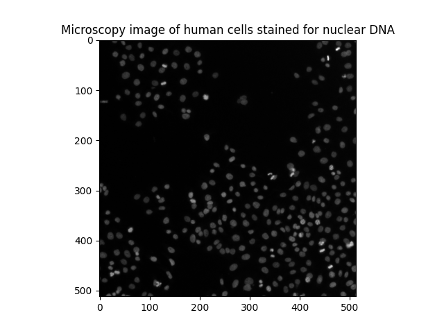
我們可以在黑暗背景上看到許多細胞核。它們大多數是平滑的,並且具有橢圓形狀。然而,我們可以區分出一些較亮的斑點,它們對應於正在進行有絲分裂(細胞分裂)的細胞核。
另一種視覺化灰階影像的方式是輪廓繪圖
fig, ax = plt.subplots(figsize=(5, 5))
qcs = ax.contour(image, origin='image')
ax.set_title('Contour plot of the same raw image')
plt.show()
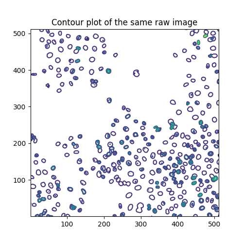
輪廓線繪製在這些層次
array([ 0., 40., 80., 120., 160., 200., 240., 280.])
每個層次分別具有以下數量的片段
# Levels without segments still contain one empty array, account for that
[len(seg) if seg[0].size else 0 for seg in qcs.allsegs]
[0, 320, 270, 48, 19, 3, 1, 0]
估計有絲分裂指數#
細胞生物學使用有絲分裂指數來量化細胞分裂,進而量化細胞增殖。根據定義,它是處於有絲分裂的細胞與細胞總數的比率。為了分析上述影像,我們對兩個閾值感興趣:一個將細胞核與背景分離,另一個將分裂細胞核(較亮的斑點)與非分裂細胞核分離。為了分離這三種不同的像素類別,我們求助於多重 Otsu 閾值處理。
thresholds = ski.filters.threshold_multiotsu(image, classes=3)
regions = np.digitize(image, bins=thresholds)

fig, ax = plt.subplots(ncols=2, figsize=(10, 5))
ax[0].imshow(image)
ax[0].set_title('Original')
ax[0].set_axis_off()
ax[1].imshow(regions)
ax[1].set_title('Multi-Otsu thresholding')
ax[1].set_axis_off()
plt.show()
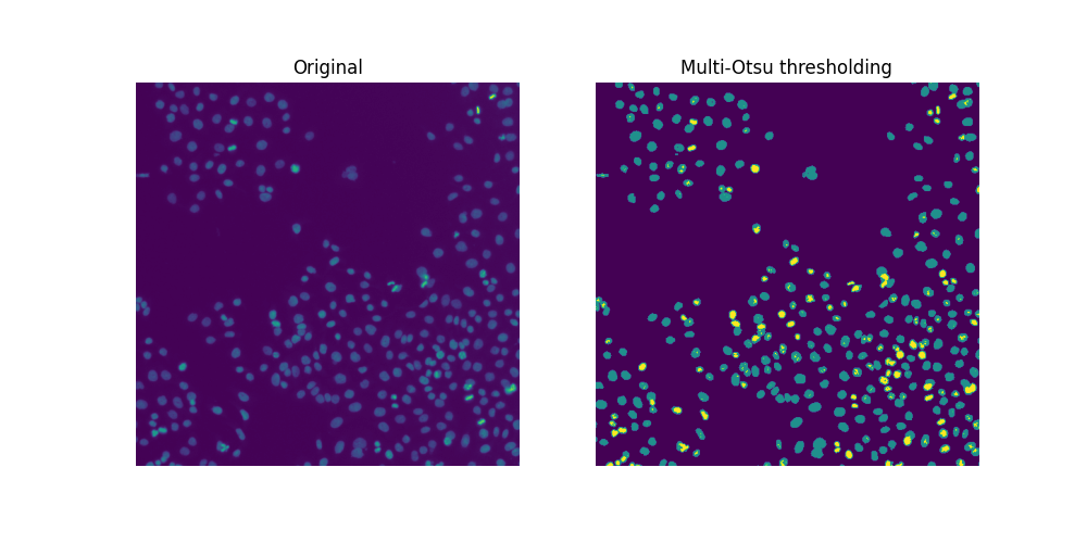
由於存在重疊的細胞核,因此僅進行閾值處理不足以分割所有細胞核。如果可以,我們可以立即計算此樣本的有絲分裂指數
cells = image > thresholds[0]
dividing = image > thresholds[1]
labeled_cells = ski.measure.label(cells)
labeled_dividing = ski.measure.label(dividing)
naive_mi = labeled_dividing.max() / labeled_cells.max()
print(naive_mi)
0.7847222222222222
哇,這不可能!分裂細胞核的數量
print(labeled_dividing.max())
226
被高估了,而細胞總數
print(labeled_cells.max())
288
被低估了。
計算分裂細胞核#
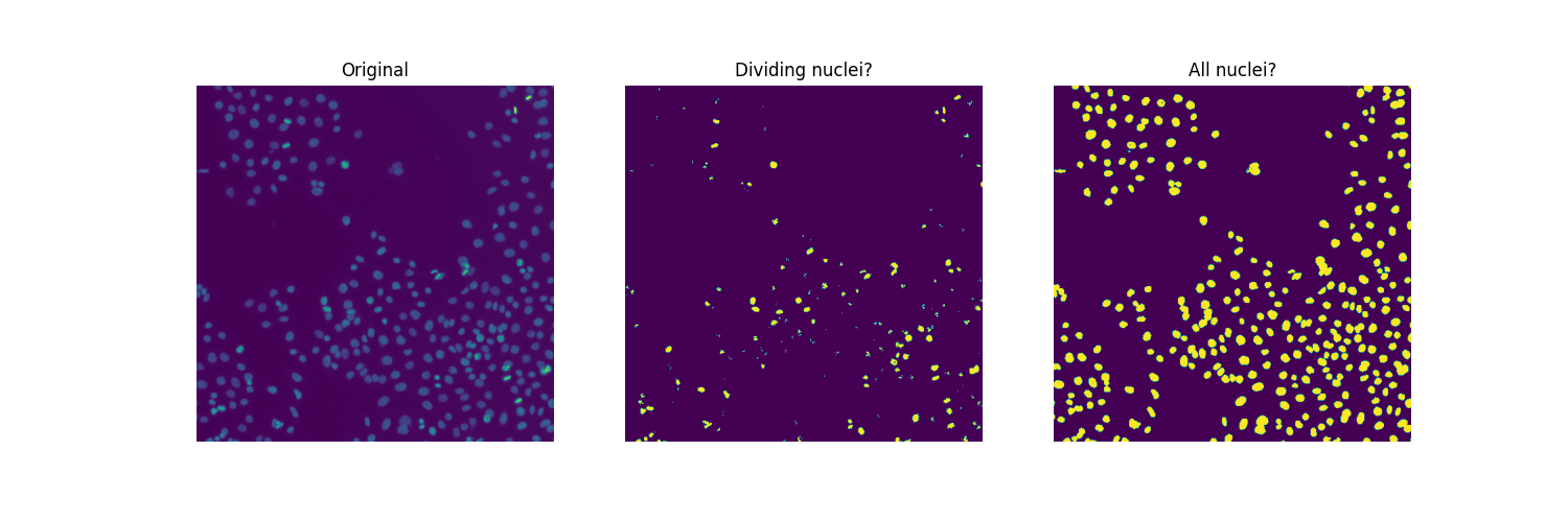
顯然,中間圖中的並非所有相連區域都是分裂細胞核。一方面,第二個閾值(thresholds[1] 的值)似乎太低,無法將那些對應於分裂細胞核的非常亮的區域與許多細胞核中存在的相對較亮的像素分開。另一方面,我們想要更平滑的影像,去除小的虛假物件,並可能合併相鄰物件的群集(有些可能對應於從一次細胞分裂中出現的兩個細胞核)。在某種程度上,我們面臨的分裂細胞核的分割挑戰與(接觸)細胞的挑戰相反。
為了找到閾值和濾波參數的合適值,我們透過二分法,以視覺方式和手動方式進行。
higher_threshold = 125
dividing = image > higher_threshold

smoother_dividing = ski.filters.rank.mean(
    ski.util.img_as_ubyte(dividing), ski.morphology.disk(4)
)

binary_smoother_dividing = smoother_dividing > 20

fig, ax = plt.subplots(figsize=(5, 5))
ax.imshow(binary_smoother_dividing)
ax.set_title('Dividing nuclei')
ax.set_axis_off()
plt.show()
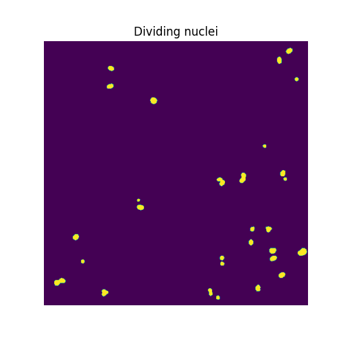
我們剩下
cleaned_dividing = ski.measure.label(binary_smoother_dividing)
print(cleaned_dividing.max())
29
此樣本中的分裂細胞核。
分割細胞核#
為了分離重疊的細胞核,我們求助於分水嶺分割。該演算法的想法是找到從一組 markers 淹沒的分水嶺盆地。我們將這些標記產生為背景距離函數的局部最大值。考慮到細胞核的典型大小,我們傳遞 min_distance=7,以便局部最大值以及標記至少間隔 7 個像素。我們還使用 exclude_border=False,以便將所有接觸影像邊界的細胞核都包括在內。
distance = ndi.distance_transform_edt(cells)

local_max_coords = ski.feature.peak_local_max(
    distance, min_distance=7, exclude_border=False
)
local_max_mask = np.zeros(distance.shape, dtype=bool)
local_max_mask[tuple(local_max_coords.T)] = True
markers = ski.measure.label(local_max_mask)

segmented_cells = ski.segmentation.watershed(-distance, markers, mask=cells)
為了方便視覺化分割結果,我們使用 color.label2rgb 函式為標記區域著色,並使用參數 bg_label=0 指定背景標籤。
fig, ax = plt.subplots(ncols=2, figsize=(10, 5))
ax[0].imshow(cells, cmap='gray')
ax[0].set_title('Overlapping nuclei')
ax[0].set_axis_off()
ax[1].imshow(ski.color.label2rgb(segmented_cells, bg_label=0))
ax[1].set_title('Segmented nuclei')
ax[1].set_axis_off()
plt.show()
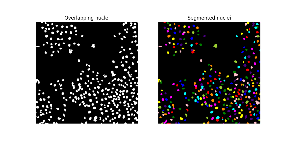
請確認分水嶺演算法已識別出更多細胞核
assert segmented_cells.max() > labeled_cells.max()
最後,我們發現此樣本中總共有
print(segmented_cells.max())
317
個細胞。因此,我們估計有絲分裂指數為
print(cleaned_dividing.max() / segmented_cells.max())
0.0914826498422713
腳本總執行時間: (0 分 3.625 秒)