直線霍夫轉換

霍夫轉換的最簡單形式是一種偵測直線的方法[1]。

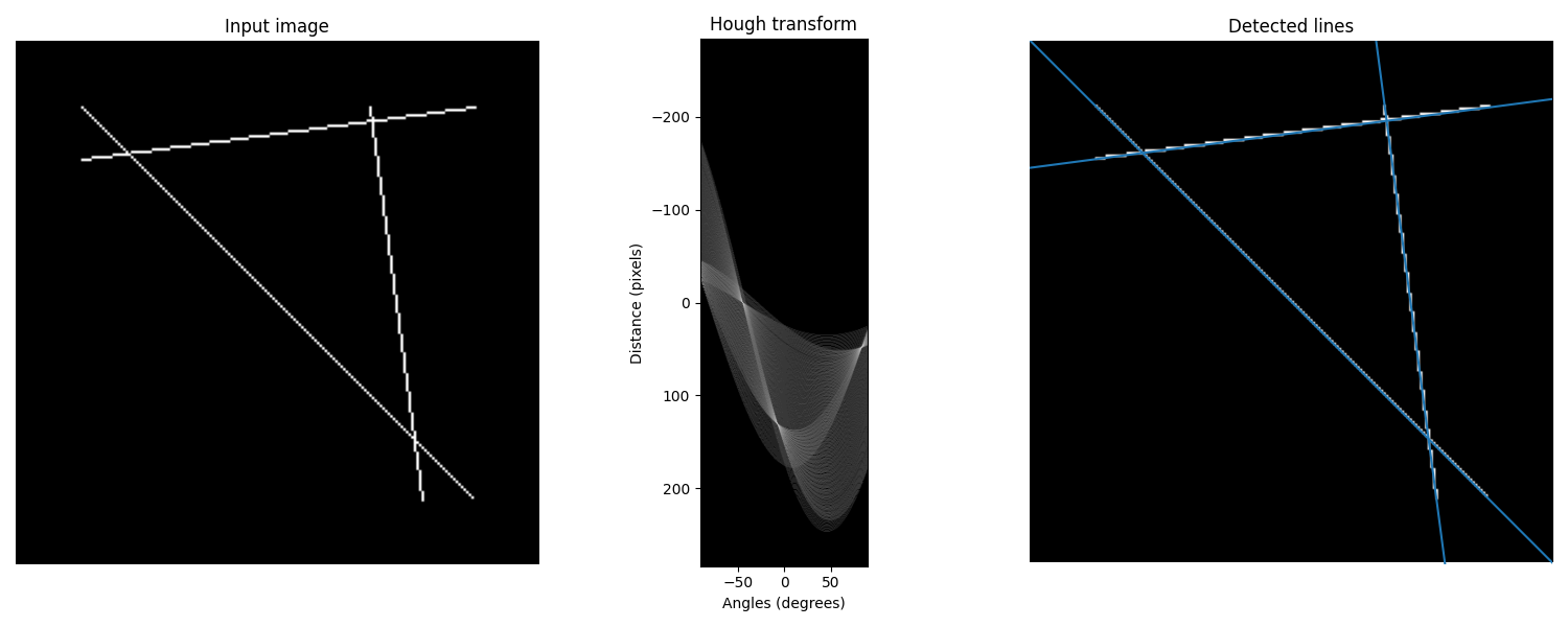
在以下範例中，我們建立一個具有直線交點的影像。然後，我們使用霍夫轉換來探索可能穿過影像的直線的參數空間。

演算法概述

通常，直線參數化為 \(y = mx + c\)，其中梯度為 \(m\)，y 軸截距為 c。然而，這表示對於垂直線，\(m\) 會趨近於無限大。因此，我們改為建構一個垂直於直線且指向原點的線段。該直線由該線段的長度 \(r\) 以及它與 x 軸形成的夾角 \(\theta\) 表示。

霍夫轉換會建構一個代表參數空間的直方圖陣列（即，對於 \(M\) 個不同的半徑值和 \(N\) 個不同的 \(\theta\) 值，則為 \(M \times N\) 矩陣）。對於每個參數組合 \(r\) 和 \(\theta\)，我們接著會找出輸入影像中會落在對應直線附近的非零像素數量，並適當地增加位置 \((r, \theta)\) 的陣列值。

我們可以將每個非零像素視為「投票」給潛在的直線候選。產生的直方圖中的局部最大值表示最有可能直線的參數。在我們的範例中，最大值出現在 45 度和 135 度，對應於每條直線的法向量角度。

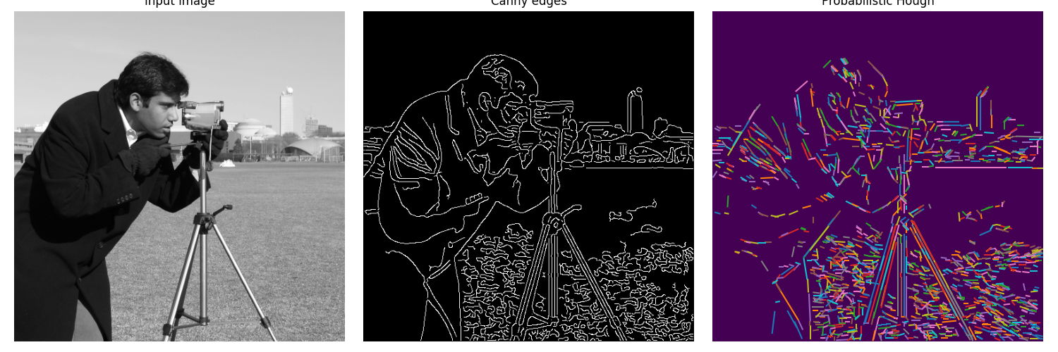
另一種方法是漸進機率霍夫轉換[2]。它基於以下假設：使用投票點的隨機子集可以很好地近似實際結果，並且可以透過沿著連接的元件行走在投票過程中提取直線。這會傳回每個線段的起點和終點，這很有用。

函式 probabilistic_hough 有三個參數：應用於霍夫累加器的通用閾值、最小線條長度和影響線條合併的線條間隙。在下面的範例中，我們找出長度大於 10 且間隙小於 3 像素的線條。

參考資料

[1]

Duda, R. O. and P. E. Hart, “Use of the Hough Transformation to Detect Lines and Curves in Pictures,” Comm. ACM, Vol. 15, pp. 11-15 (January, 1972)

[2]

C. Galamhos, J. Matas and J. Kittler,”Progressive probabilistic Hough transform for line detection”, in IEEE Computer Society Conference on Computer Vision and Pattern Recognition, 1999.

直線霍夫轉換

import numpy as np

from skimage.transform import hough_line, hough_line_peaks
from skimage.feature import canny
from skimage.draw import line as draw_line
from skimage import data

import matplotlib.pyplot as plt
from matplotlib import cm


# Constructing test image
image = np.zeros((200, 200))
idx = np.arange(25, 175)
image[idx, idx] = 255
image[draw_line(45, 25, 25, 175)] = 255
image[draw_line(25, 135, 175, 155)] = 255

# Classic straight-line Hough transform
# Set a precision of 0.5 degree.
tested_angles = np.linspace(-np.pi / 2, np.pi / 2, 360, endpoint=False)
h, theta, d = hough_line(image, theta=tested_angles)

# Generating figure 1
fig, axes = plt.subplots(1, 3, figsize=(15, 6))
ax = axes.ravel()

ax[0].imshow(image, cmap=cm.gray)
ax[0].set_title('Input image')
ax[0].set_axis_off()

angle_step = 0.5 * np.diff(theta).mean()
d_step = 0.5 * np.diff(d).mean()
bounds = [
    np.rad2deg(theta[0] - angle_step),
    np.rad2deg(theta[-1] + angle_step),
    d[-1] + d_step,
    d[0] - d_step,
]
ax[1].imshow(np.log(1 + h), extent=bounds, cmap=cm.gray, aspect=1 / 1.5)
ax[1].set_title('Hough transform')
ax[1].set_xlabel('Angles (degrees)')
ax[1].set_ylabel('Distance (pixels)')
ax[1].axis('image')

ax[2].imshow(image, cmap=cm.gray)
ax[2].set_ylim((image.shape[0], 0))
ax[2].set_axis_off()
ax[2].set_title('Detected lines')

for _, angle, dist in zip(*hough_line_peaks(h, theta, d)):
    (x0, y0) = dist * np.array([np.cos(angle), np.sin(angle)])
    ax[2].axline((x0, y0), slope=np.tan(angle + np.pi / 2))

plt.tight_layout()
plt.show()

機率霍夫轉換

from skimage.transform import probabilistic_hough_line

# Line finding using the Probabilistic Hough Transform
image = data.camera()
edges = canny(image, 2, 1, 25)
lines = probabilistic_hough_line(edges, threshold=10, line_length=5, line_gap=3)

# Generating figure 2
fig, axes = plt.subplots(1, 3, figsize=(15, 5), sharex=True, sharey=True)
ax = axes.ravel()

ax[0].imshow(image, cmap=cm.gray)
ax[0].set_title('Input image')

ax[1].imshow(edges, cmap=cm.gray)
ax[1].set_title('Canny edges')

ax[2].imshow(edges * 0)
for line in lines:
    p0, p1 = line
    ax[2].plot((p0[0], p1[0]), (p0[1], p1[1]))
ax[2].set_xlim((0, image.shape[1]))
ax[2].set_ylim((image.shape[0], 0))
ax[2].set_title('Probabilistic Hough')

for a in ax:
    a.set_axis_off()

plt.tight_layout()
plt.show()