Flood Fill (填滿)

Flood Fill (填滿) 是一種演算法，用於根據影像中與初始種子點相似的值來識別和/或變更相鄰值 [1]。概念上的類比是許多圖形編輯器中的「油漆桶」工具。

[1]

https://en.wikipedia.org/wiki/Flood_fill

基本範例

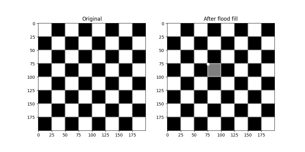
首先，一個基本範例，我們將把棋盤格正方形從白色變更為中灰色。

import numpy as np
import matplotlib.pyplot as plt
from skimage import data, filters, color, morphology
from skimage.segmentation import flood, flood_fill


checkers = data.checkerboard()

# Fill a square near the middle with value 127, starting at index (76, 76)
filled_checkers = flood_fill(checkers, (76, 76), 127)

fig, ax = plt.subplots(ncols=2, figsize=(10, 5))

ax[0].imshow(checkers, cmap=plt.cm.gray)
ax[0].set_title('Original')

ax[1].imshow(filled_checkers, cmap=plt.cm.gray)
ax[1].plot(76, 76, 'wo')  # seed point
ax[1].set_title('After flood fill')

plt.show()

進階範例

由於標準 Flood Fill (填滿) 需要相鄰像素嚴格相等，因此它在具有色彩漸變和雜訊的真實世界影像上的用途有限。tolerance 關鍵字引數擴大了初始值周圍允許的範圍，允許在真實世界影像上使用。

在這裡，我們將在攝影師身上做一些實驗。首先，將他的外套從深色變成淺色。

cameraman = data.camera()

# Change the cameraman's coat from dark to light (255).  The seed point is
# chosen as (155, 150)
light_coat = flood_fill(cameraman, (155, 150), 255, tolerance=10)
fig, ax = plt.subplots(ncols=2, figsize=(10, 5))

ax[0].imshow(cameraman, cmap=plt.cm.gray)
ax[0].set_title('Original')
ax[0].axis('off')

ax[1].imshow(light_coat, cmap=plt.cm.gray)
ax[1].plot(150, 155, 'ro')  # seed point
ax[1].set_title('After flood fill')
ax[1].axis('off')

plt.show()

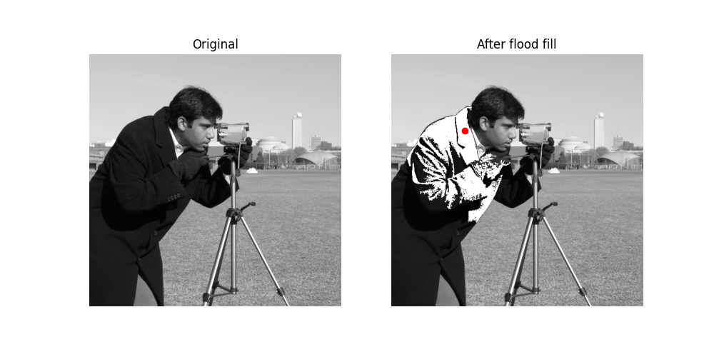
攝影師的外套有不同的灰色陰影。只有與種子值附近陰影匹配的外套部分會被變更。

容差實驗

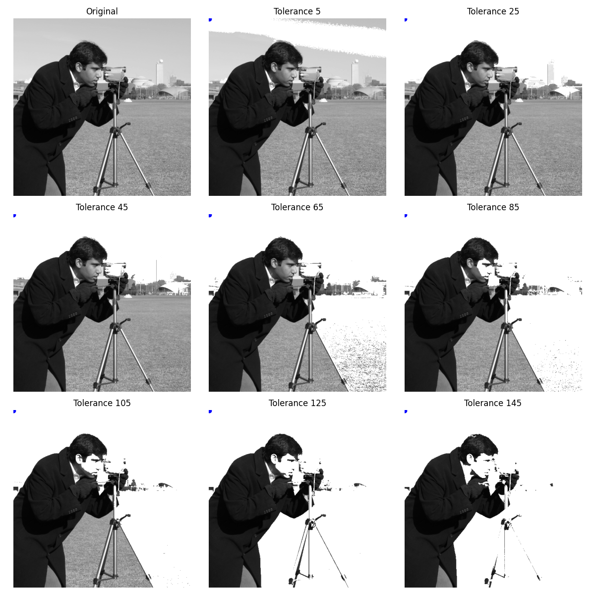
為了更好地直觀了解容差參數如何運作，以下是一組影像，逐步增加參數，且種子點位於左上角。

output = []

for i in range(8):
    tol = 5 + 20 * i
    output.append(flood_fill(cameraman, (0, 0), 255, tolerance=tol))

# Initialize plot and place original image
fig, ax = plt.subplots(nrows=3, ncols=3, figsize=(12, 12))
ax[0, 0].imshow(cameraman, cmap=plt.cm.gray)
ax[0, 0].set_title('Original')
ax[0, 0].axis('off')

# Plot all eight different tolerances for comparison.
for i in range(8):
    m, n = np.unravel_index(i + 1, (3, 3))
    ax[m, n].imshow(output[i], cmap=plt.cm.gray)
    ax[m, n].set_title(f'Tolerance {5 + 20 * i}')
    ax[m, n].axis('off')
    ax[m, n].plot(0, 0, 'bo')  # seed point

fig.tight_layout()
plt.show()

Flood (填滿) 作為遮罩

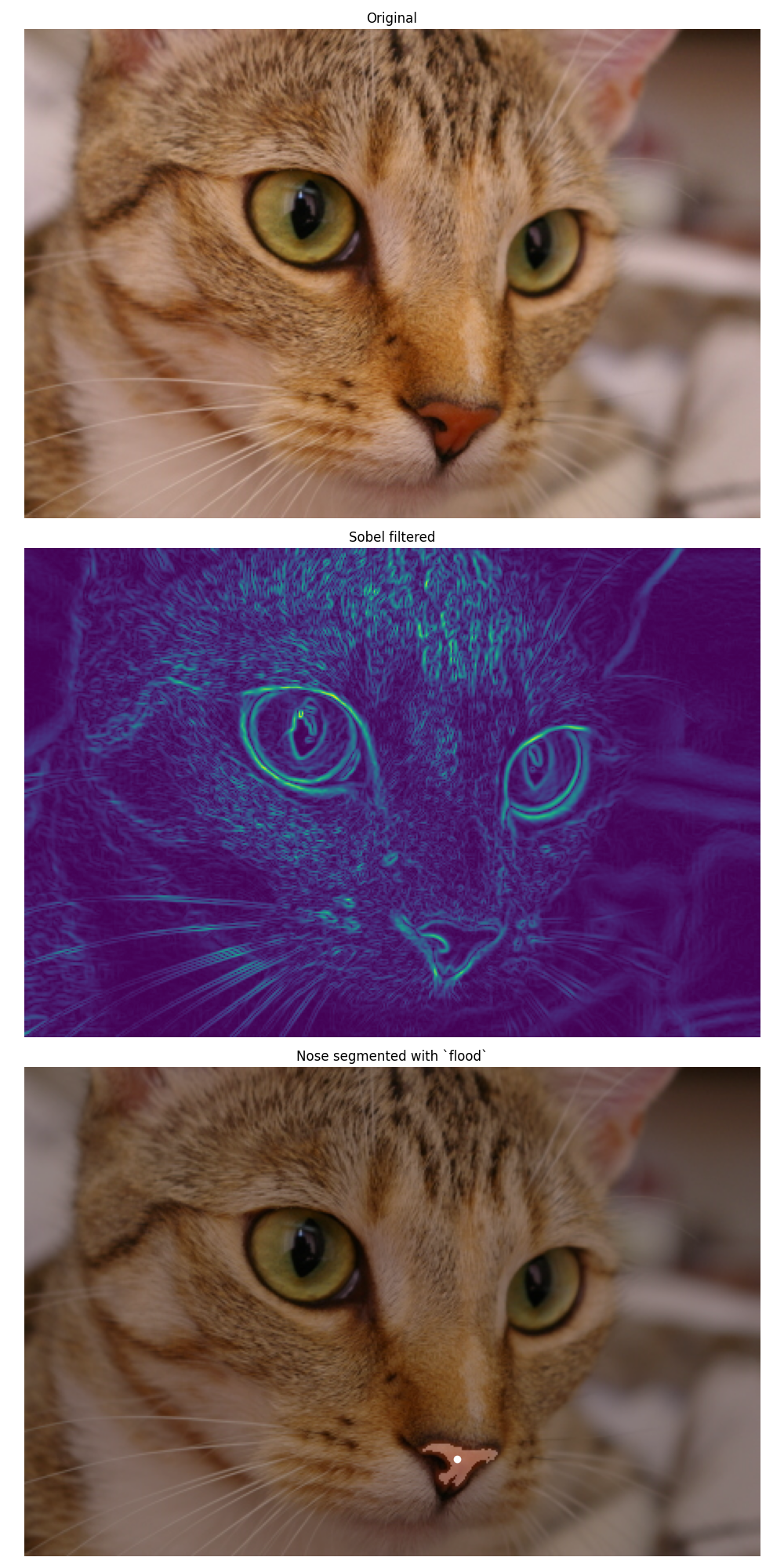
有一個姊妹函式 flood 可用，它會傳回一個遮罩，用於識別 Flood (填滿) 區域，而不是修改影像本身。這對於分割目的和更進階的分析管線非常有用。

在這裡，我們分割貓的鼻子。然而，Flood[_fill] 不支援多通道影像。相反，我們對紅色通道進行 Sobel 濾波以增強邊緣，然後以容差對鼻子進行 Flood (填滿)。

cat = data.chelsea()
cat_sobel = filters.sobel(cat[..., 0])
cat_nose = flood(cat_sobel, (240, 265), tolerance=0.03)

fig, ax = plt.subplots(nrows=3, figsize=(10, 20))

ax[0].imshow(cat)
ax[0].set_title('Original')
ax[0].axis('off')

ax[1].imshow(cat_sobel)
ax[1].set_title('Sobel filtered')
ax[1].axis('off')

ax[2].imshow(cat)
ax[2].imshow(cat_nose, cmap=plt.cm.gray, alpha=0.3)
ax[2].plot(265, 240, 'wo')  # seed point
ax[2].set_title('Nose segmented with `flood`')
ax[2].axis('off')

fig.tight_layout()
plt.show()

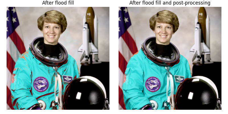
HSV 空間中的 Flood Fill (填滿) 和遮罩後處理

由於 Flood Fill (填滿) 在單通道影像上運作，我們在此將影像轉換為 HSV（色相、飽和度、數值）空間，以便對相似色相的像素進行 Flood (填滿)。

在此範例中，我們也展示了可以透過 skimage.segmentation.flood() 傳回的二元遮罩進行後處理，這要歸功於 skimage.morphology 的函式。

img = data.astronaut()
img_hsv = color.rgb2hsv(img)
img_hsv_copy = np.copy(img_hsv)

# flood function returns a mask of flooded pixels
mask = flood(img_hsv[..., 0], (313, 160), tolerance=0.016)
# Set pixels of mask to new value for hue channel
img_hsv[mask, 0] = 0.5
# Post-processing in order to improve the result
# Remove white pixels from flag, using saturation channel
mask_postprocessed = np.logical_and(mask, img_hsv_copy[..., 1] > 0.4)
# Remove thin structures with binary opening
mask_postprocessed = morphology.binary_opening(mask_postprocessed, np.ones((3, 3)))
# Fill small holes with binary closing
mask_postprocessed = morphology.binary_closing(mask_postprocessed, morphology.disk(20))
img_hsv_copy[mask_postprocessed, 0] = 0.5

fig, ax = plt.subplots(1, 2, figsize=(8, 4))
ax[0].imshow(color.hsv2rgb(img_hsv))
ax[0].axis('off')
ax[0].set_title('After flood fill')
ax[1].imshow(color.hsv2rgb(img_hsv_copy))
ax[1].axis('off')
ax[1].set_title('After flood fill and post-processing')

fig.tight_layout()
plt.show()