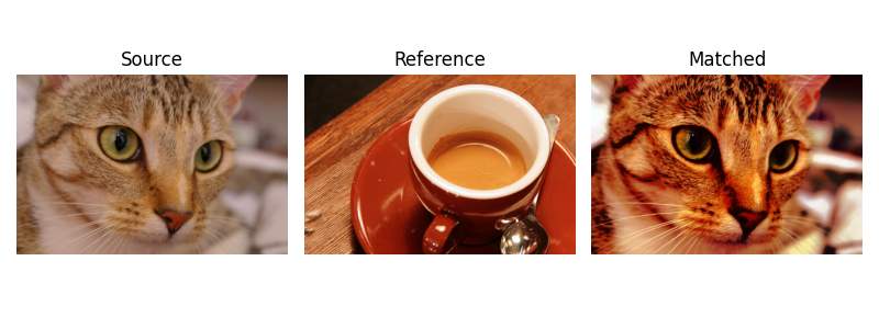
直方圖匹配

此範例示範直方圖匹配的功能。它會操作輸入影像的像素，使其直方圖與參考影像的直方圖匹配。如果影像有多個通道，則每個通道會獨立進行匹配，只要輸入影像和參考影像的通道數相等即可。

直方圖匹配可以用作影像處理的輕量級正規化，例如特徵匹配，尤其是在影像來自不同來源或在不同條件（即光照）下拍攝的情況下。

import matplotlib.pyplot as plt

from skimage import data
from skimage import exposure
from skimage.exposure import match_histograms

reference = data.coffee()
image = data.chelsea()

matched = match_histograms(image, reference, channel_axis=-1)

fig, (ax1, ax2, ax3) = plt.subplots(
    nrows=1, ncols=3, figsize=(8, 3), sharex=True, sharey=True
)
for aa in (ax1, ax2, ax3):
    aa.set_axis_off()

ax1.imshow(image)
ax1.set_title('Source')
ax2.imshow(reference)
ax2.set_title('Reference')
ax3.imshow(matched)
ax3.set_title('Matched')

plt.tight_layout()
plt.show()

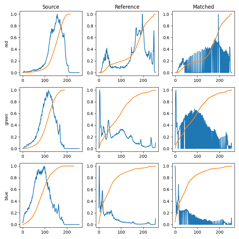
為了說明直方圖匹配的效果，我們繪製每個 RGB 通道的直方圖和累積直方圖。顯然，匹配的影像對於每個通道都具有與參考影像相同的累積直方圖。

fig, axes = plt.subplots(nrows=3, ncols=3, figsize=(8, 8))


for i, img in enumerate((image, reference, matched)):
    for c, c_color in enumerate(('red', 'green', 'blue')):
        img_hist, bins = exposure.histogram(img[..., c], source_range='dtype')
        axes[c, i].plot(bins, img_hist / img_hist.max())
        img_cdf, bins = exposure.cumulative_distribution(img[..., c])
        axes[c, i].plot(bins, img_cdf)
        axes[c, 0].set_ylabel(c_color)

axes[0, 0].set_title('Source')
axes[0, 1].set_title('Reference')
axes[0, 2].set_title('Matched')

plt.tight_layout()
plt.show()