圓形和橢圓形霍夫變換

霍夫變換的最簡單形式是一種偵測直線的方法，但它也可以用於偵測圓形或橢圓形。該演算法假設邊緣已被偵測到，並且對雜訊或遺失的點具有穩健性。

圓形偵測

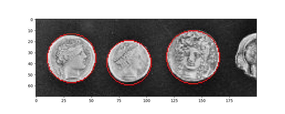
在以下範例中，霍夫變換用於偵測硬幣位置並比對其邊緣。我們提供了一系列合理的半徑。對於每個半徑，擷取兩個圓形，最後保留五個最突出的候選者。結果顯示硬幣位置已被良好偵測到。

演算法概述

給定白色背景上的黑色圓形，我們先猜測其半徑（或一系列半徑）以建構一個新的圓形。此圓形應用於原始圖片的每個黑色像素，並且此圓形的座標在累加器中投票。從這種幾何結構來看，原始圓形中心位置會獲得最高分。

請注意，累加器的大小被建構成大於原始圖片，以便偵測框架外的中心。其大小擴展為較大半徑的兩倍。

import numpy as np
import matplotlib.pyplot as plt

from skimage import data, color
from skimage.transform import hough_circle, hough_circle_peaks
from skimage.feature import canny
from skimage.draw import circle_perimeter
from skimage.util import img_as_ubyte


# Load picture and detect edges
image = img_as_ubyte(data.coins()[160:230, 70:270])
edges = canny(image, sigma=3, low_threshold=10, high_threshold=50)


# Detect two radii
hough_radii = np.arange(20, 35, 2)
hough_res = hough_circle(edges, hough_radii)

# Select the most prominent 3 circles
accums, cx, cy, radii = hough_circle_peaks(hough_res, hough_radii, total_num_peaks=3)

# Draw them
fig, ax = plt.subplots(ncols=1, nrows=1, figsize=(10, 4))
image = color.gray2rgb(image)
for center_y, center_x, radius in zip(cy, cx, radii):
    circy, circx = circle_perimeter(center_y, center_x, radius, shape=image.shape)
    image[circy, circx] = (220, 20, 20)

ax.imshow(image, cmap=plt.cm.gray)
plt.show()

橢圓形偵測

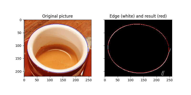
在第二個範例中，目的是偵測咖啡杯的邊緣。基本上，這是圓形的投影，即橢圓形。要解決的問題要困難得多，因為必須確定五個參數，而不是圓形的三個參數。

演算法概述

該演算法採用屬於橢圓形的兩個不同點。它假設這兩個點形成長軸。所有其他點的迴圈確定候選橢圓的短軸長度。如果足夠多的「有效」候選者具有相似的短軸長度，則後者會包含在結果中。所謂有效，是指短軸和長軸長度都在規定的範圍內。有關該演算法的完整描述，請參閱參考文獻[1]。

參考文獻

[1]

Xie, Yonghong, and Qiang Ji. “A new efficient ellipse detection method.” Pattern Recognition, 2002. Proceedings. 16th International Conference on. Vol. 2. IEEE, 2002

import matplotlib.pyplot as plt

from skimage import data, color, img_as_ubyte
from skimage.feature import canny
from skimage.transform import hough_ellipse
from skimage.draw import ellipse_perimeter

# Load picture, convert to grayscale and detect edges
image_rgb = data.coffee()[0:220, 160:420]
image_gray = color.rgb2gray(image_rgb)
edges = canny(image_gray, sigma=2.0, low_threshold=0.55, high_threshold=0.8)

# Perform a Hough Transform
# The accuracy corresponds to the bin size of the histogram for minor axis lengths.
# A higher `accuracy` value will lead to more ellipses being found, at the
# cost of a lower precision on the minor axis length estimation.
# A higher `threshold` will lead to less ellipses being found, filtering out those
# with fewer edge points (as found above by the Canny detector) on their perimeter.
result = hough_ellipse(edges, accuracy=20, threshold=250, min_size=100, max_size=120)
result.sort(order='accumulator')

# Estimated parameters for the ellipse
best = list(result[-1])
yc, xc, a, b = (int(round(x)) for x in best[1:5])
orientation = best[5]

# Draw the ellipse on the original image
cy, cx = ellipse_perimeter(yc, xc, a, b, orientation)
image_rgb[cy, cx] = (0, 0, 255)
# Draw the edge (white) and the resulting ellipse (red)
edges = color.gray2rgb(img_as_ubyte(edges))
edges[cy, cx] = (250, 0, 0)

fig2, (ax1, ax2) = plt.subplots(
    ncols=2, nrows=1, figsize=(8, 4), sharex=True, sharey=True
)

ax1.set_title('Original picture')
ax1.imshow(image_rgb)

ax2.set_title('Edge (white) and result (red)')
ax2.imshow(edges)

plt.show()