形態學濾波

形態學影像處理是一組非線性操作，與影像中特徵的形狀或形態相關，例如邊界、骨架等。在任何給定的技術中，我們使用稱為結構元素的小形狀或範本探測影像，該結構元素定義像素周圍的感興趣區域或鄰域。

在本文件中，我們概述了以下基本形態學操作

1. 侵蝕

2. 膨脹

3. 開運算

4. 閉運算

5. 白色頂帽

6. 黑色頂帽

7. 骨架化

8. 凸包

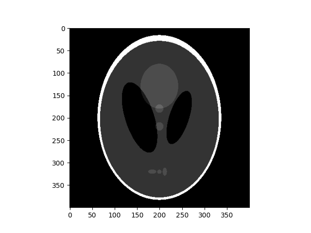
首先，讓我們使用 io.imread 載入影像。請注意，形態學函數僅適用於灰階或二元影像，因此我們設定 as_gray=True。

import matplotlib.pyplot as plt
from skimage import data
from skimage.util import img_as_ubyte

orig_phantom = img_as_ubyte(data.shepp_logan_phantom())
fig, ax = plt.subplots()
ax.imshow(orig_phantom, cmap=plt.cm.gray)

<matplotlib.image.AxesImage object at 0x7f036a3059a0>

我們也來定義一個用於繪製比較的方便函數

def plot_comparison(original, filtered, filter_name):
    fig, (ax1, ax2) = plt.subplots(ncols=2, figsize=(8, 4), sharex=True, sharey=True)
    ax1.imshow(original, cmap=plt.cm.gray)
    ax1.set_title('original')
    ax1.set_axis_off()
    ax2.imshow(filtered, cmap=plt.cm.gray)
    ax2.set_title(filter_name)
    ax2.set_axis_off()

侵蝕

形態學 侵蝕 將 (i, j) 處的像素設定為以 (i, j) 為中心的所有鄰域像素的最小值。傳遞給 侵蝕 的結構元素 足跡 是一個布林值陣列，用於描述此鄰域。在下面，我們使用 disk 建立一個圓形結構元素，我們將其用於以下大多數範例。

from skimage.morphology import erosion, dilation, opening, closing, white_tophat
from skimage.morphology import black_tophat, skeletonize, convex_hull_image
from skimage.morphology import disk

footprint = disk(6)
eroded = erosion(orig_phantom, footprint)
plot_comparison(orig_phantom, eroded, 'erosion')

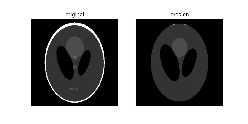
請注意，隨著我們增加磁碟的大小，影像的白色邊界如何消失或被侵蝕。另請注意中心兩個黑色橢圓形的大小增加，以及影像下半部分 3 個淺灰色色塊的消失。

膨脹

形態學 膨脹 將 (i, j) 處的像素設定為以 (i, j) 為中心的所有鄰域像素的最大值。膨脹會擴大明亮區域並縮小黑暗區域。

dilated = dilation(orig_phantom, footprint)
plot_comparison(orig_phantom, dilated, 'dilation')

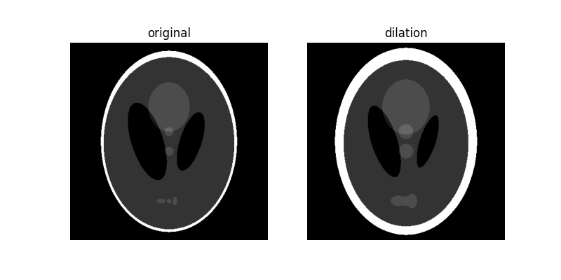
請注意，隨著我們增加磁碟的大小，影像的白色邊界如何加厚或膨脹。另請注意中心兩個黑色橢圓形的大小減小，以及中心淺灰色圓形和影像下半部分 3 個色塊的加厚。

開運算

影像的形態學 開運算 定義為先侵蝕再膨脹。開運算可以移除小的明亮斑點（即「鹽」），並連接小的黑暗裂縫。

opened = opening(orig_phantom, footprint)
plot_comparison(orig_phantom, opened, 'opening')

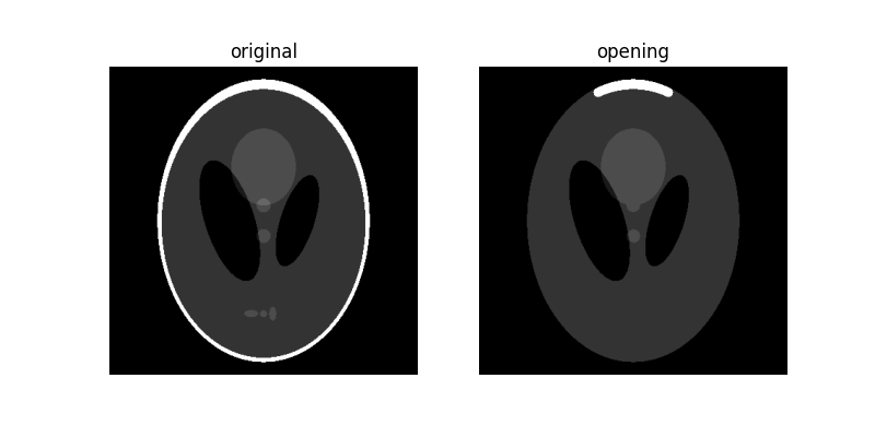
由於 開運算 影像從侵蝕操作開始，因此小於結構元素的明亮區域會被移除。隨後的膨脹操作可確保大於結構元素的明亮區域保留其原始大小。請注意，中心的亮暗形狀如何保留其原始厚度，但底部的 3 個較淺的色塊被完全侵蝕。外部白色環突出顯示了大小依賴性：比結構元素薄的環部分被完全擦除，而頂部較厚的區域保留其原始厚度。

閉運算

影像的形態學 閉運算 定義為先膨脹再侵蝕。閉運算可以移除小的黑暗斑點（即「胡椒」），並連接小的明亮裂縫。

為了更清楚地說明這一點，讓我們在白色邊框上新增一個小裂縫

phantom = orig_phantom.copy()
phantom[10:30, 200:210] = 0

closed = closing(phantom, footprint)
plot_comparison(phantom, closed, 'closing')

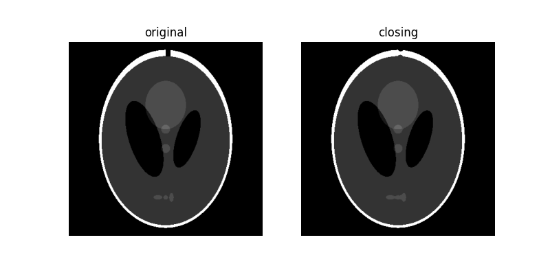
由於 閉運算 影像從膨脹操作開始，因此小於結構元素的黑暗區域會被移除。隨後的侵蝕操作可確保大於結構元素的黑暗區域保留其原始大小。請注意，底部的白色橢圓形如何因膨脹而連接，但其他黑暗區域保留其原始大小。另請注意，我們新增的裂縫大多已被移除。

白色頂帽

影像的 white_tophat 定義為影像減去其形態學開運算。此操作會傳回小於結構元素的影像明亮斑點。

為了讓事情更有趣，我們將在影像中新增明亮和黑暗的斑點

phantom = orig_phantom.copy()
phantom[340:350, 200:210] = 255
phantom[100:110, 200:210] = 0

w_tophat = white_tophat(phantom, footprint)
plot_comparison(phantom, w_tophat, 'white tophat')

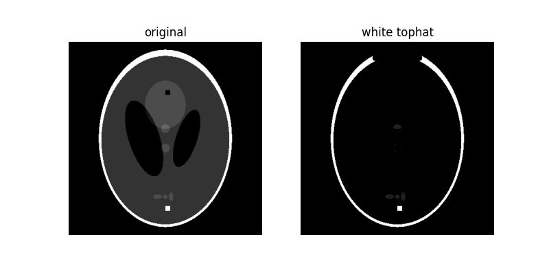
如您所見，由於 10 像素寬的白色正方形小於結構元素，因此被突出顯示。此外，橢圓形周圍的大部分細白色邊緣也被保留，因為它們小於結構元素，但頂部較厚的區域則消失了。

黑色頂帽

影像的 black_tophat 定義為其形態學的閉運算減去原始影像。此操作會回傳影像中比結構元素小的暗點。

b_tophat = black_tophat(phantom, footprint)
plot_comparison(phantom, b_tophat, 'black tophat')

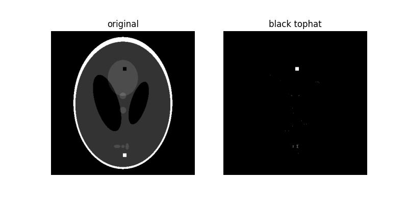
如您所見，由於 10 像素寬的黑色正方形小於結構元素，因此被突出顯示。

對偶性

您應該已經注意到，許多這些操作只是另一個操作的反向。這種對偶性可以總結如下：

1. 侵蝕 <-> 膨脹

2. 開運算 <-> 閉運算

3. 白色頂帽 <-> 黑色頂帽

骨架化

細化用於將二值影像中的每個連通組件縮減為單像素寬的骨架。重要的是要注意，這僅在二值影像上執行。

horse = data.horse()

sk = skeletonize(horse == 0)
plot_comparison(horse, sk, 'skeletonize')

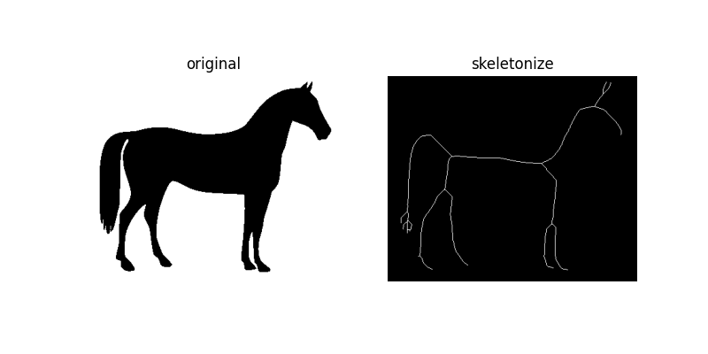
顧名思義，此技術透過連續應用細化來將影像細化為 1 像素寬的骨架。

凸包

convex_hull_image 是包含在最小凸多邊形內的像素集合，該多邊形包圍輸入影像中的所有白色像素。再次注意，這也是在二值影像上執行的。

hull1 = convex_hull_image(horse == 0)
plot_comparison(horse, hull1, 'convex hull')

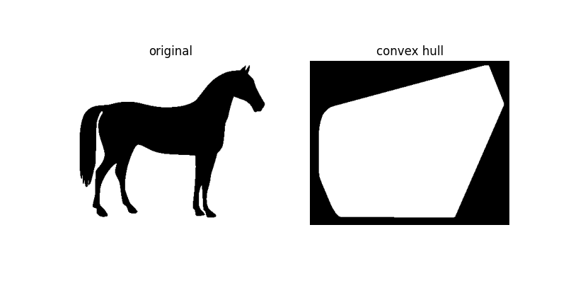
如圖所示，convex_hull_image 會給出覆蓋影像中白色或 True 的最小多邊形。

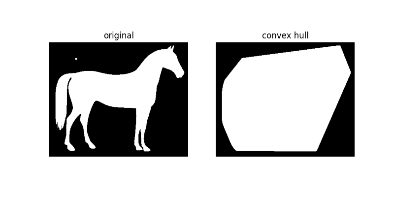
如果我們在影像中新增一個小顆粒，我們可以觀察凸包如何適應以包圍該顆粒。

horse_mask = horse == 0
horse_mask[45:50, 75:80] = 1

hull2 = convex_hull_image(horse_mask)
plot_comparison(horse_mask, hull2, 'convex hull')

其他資源

1. MathWorks 關於形態學處理的教學

2. 奧克蘭大學關於形態學影像處理的教學

3. https://en.wikipedia.org/wiki/Mathematical_morphology

plt.show()