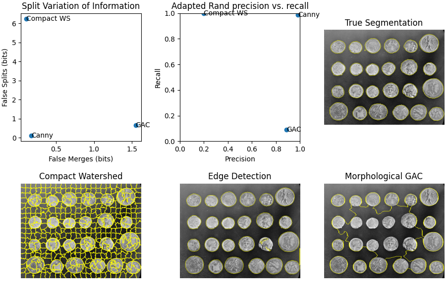
評估分割指標

當嘗試不同的分割方法時，您如何知道哪一種最好？如果您有真實值或黃金標準分割，您可以使用各種指標來檢查每種自動方法與真實值的接近程度。在本範例中，我們使用一個易於分割的影像作為範例，說明如何解釋各種分割指標。我們將使用調整後的蘭德錯誤和資訊變異作為範例指標，並觀察過度分割 (將真實分割分割成太多子分割) 和分割不足 (將不同的真實分割合併為單一分割) 如何影響不同的分數。

import numpy as np
import matplotlib.pyplot as plt
from scipy import ndimage as ndi

from skimage import data
from skimage.metrics import adapted_rand_error, variation_of_information
from skimage.filters import sobel
from skimage.measure import label
from skimage.util import img_as_float
from skimage.feature import canny
from skimage.morphology import remove_small_objects
from skimage.segmentation import (
    morphological_geodesic_active_contour,
    inverse_gaussian_gradient,
    watershed,
    mark_boundaries,
)

image = data.coins()

首先，我們產生真實分割。對於這個簡單的影像，我們知道將產生完美分割的確切函數和參數。在真實情況下，您通常會透過手動註解或分割的「繪製」來產生真實值。

elevation_map = sobel(image)
markers = np.zeros_like(image)
markers[image < 30] = 1
markers[image > 150] = 2
im_true = watershed(elevation_map, markers)
im_true = ndi.label(ndi.binary_fill_holes(im_true - 1))[0]

接下來，我們建立三個具有不同特性的不同分割。第一個使用具有緊湊度的skimage.segmentation.watershed()，這是一個有用的初始分割，但作為最終結果太過精細。我們將看到這如何導致過度分割指標飆升。

edges = sobel(image)
im_test1 = watershed(edges, markers=468, compactness=0.001)

下一個方法使用 Canny 邊緣濾波器，skimage.feature.canny()。這是一個非常好的邊緣尋找器，並且提供了平衡的結果。

edges = canny(image)
fill_coins = ndi.binary_fill_holes(edges)
im_test2 = ndi.label(remove_small_objects(fill_coins, 21))[0]

最後，我們使用形態測地線主動輪廓，skimage.segmentation.morphological_geodesic_active_contour()，這是一種通常會產生良好結果的方法，但需要很長時間才能收斂到一個好的答案。我們故意在 100 次迭代時縮短程序，以便最終結果分割不足，這意味著許多區域合併為一個分割。我們將看到分割指標的相應影響。

image = img_as_float(image)
gradient = inverse_gaussian_gradient(image)
init_ls = np.zeros(image.shape, dtype=np.int8)
init_ls[10:-10, 10:-10] = 1
im_test3 = morphological_geodesic_active_contour(
    gradient,
    num_iter=100,
    init_level_set=init_ls,
    smoothing=1,
    balloon=-1,
    threshold=0.69,
)
im_test3 = label(im_test3)

method_names = [
    'Compact watershed',
    'Canny filter',
    'Morphological Geodesic Active Contours',
]
short_method_names = ['Compact WS', 'Canny', 'GAC']

precision_list = []
recall_list = []
split_list = []
merge_list = []
for name, im_test in zip(method_names, [im_test1, im_test2, im_test3]):
    error, precision, recall = adapted_rand_error(im_true, im_test)
    splits, merges = variation_of_information(im_true, im_test)
    split_list.append(splits)
    merge_list.append(merges)
    precision_list.append(precision)
    recall_list.append(recall)
    print(f'\n## Method: {name}')
    print(f'Adapted Rand error: {error}')
    print(f'Adapted Rand precision: {precision}')
    print(f'Adapted Rand recall: {recall}')
    print(f'False Splits: {splits}')
    print(f'False Merges: {merges}')

fig, axes = plt.subplots(2, 3, figsize=(9, 6), constrained_layout=True)
ax = axes.ravel()

ax[0].scatter(merge_list, split_list)
for i, txt in enumerate(short_method_names):
    ax[0].annotate(txt, (merge_list[i], split_list[i]), verticalalignment='center')
ax[0].set_xlabel('False Merges (bits)')
ax[0].set_ylabel('False Splits (bits)')
ax[0].set_title('Split Variation of Information')

ax[1].scatter(precision_list, recall_list)
for i, txt in enumerate(short_method_names):
    ax[1].annotate(txt, (precision_list[i], recall_list[i]), verticalalignment='center')
ax[1].set_xlabel('Precision')
ax[1].set_ylabel('Recall')
ax[1].set_title('Adapted Rand precision vs. recall')
ax[1].set_xlim(0, 1)
ax[1].set_ylim(0, 1)

ax[2].imshow(mark_boundaries(image, im_true))
ax[2].set_title('True Segmentation')
ax[2].set_axis_off()

ax[3].imshow(mark_boundaries(image, im_test1))
ax[3].set_title('Compact Watershed')
ax[3].set_axis_off()

ax[4].imshow(mark_boundaries(image, im_test2))
ax[4].set_title('Edge Detection')
ax[4].set_axis_off()

ax[5].imshow(mark_boundaries(image, im_test3))
ax[5].set_title('Morphological GAC')
ax[5].set_axis_off()

plt.show()

## Method: Compact watershed
Adapted Rand error: 0.6696040824674964
Adapted Rand precision: 0.19789866776616444
Adapted Rand recall: 0.999747618854942
False Splits: 6.235700763571577
False Merges: 0.10855347108404328

## Method: Canny filter
Adapted Rand error: 0.01477976422795424
Adapted Rand precision: 0.9829789913922441
Adapted Rand recall: 0.9874717238207291
False Splits: 0.11790842956314956
False Merges: 0.17056628682718059

## Method: Morphological Geodesic Active Contours
Adapted Rand error: 0.8380351755097508
Adapted Rand precision: 0.8878701134692834
Adapted Rand recall: 0.08911012454398565
False Splits: 0.6563768831046463
False Merges: 1.5482985465714199